Shuai-Agarwal turbulence Model

From CFD-Wiki

Introduction

One-equation k-kL turbulence model was developed from two-equation k-kL closure of Abdol-Hamid et al. Improvements to the original formulation of one-equation k-kL model (AIAA 2019-1879) were made by optimizing the model constants (AIAA 2020-1075). The new improved model has been validated by simulating several benchmark canonical wall-bounded turbulent flows with small regions of separation from NASA TMR (https://turbmodels.larc.nasa.gov/). The model needs further investigations by the scientific community to evaluate its potential.

Shuai – Agarwal One Equation k-kL Turbulence Model

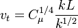
The turbulent kinematic viscosity is given by:

$v_{t}=C_{\mu}^{1/4} \frac{kL}{{k}^{1/2}}$

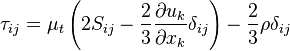
The final form of the new Shuai-Agarwal one-equation k-kL model is obtained as:

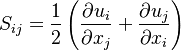
$\frac{D v_{t}}{D t}=a_{1}\left(C_{\phi 1}-\frac{1}{2}\right) \frac{P}{S}+\left(\frac{1}{2} a_{1}-\frac{C_{\phi 2}}{\sqrt{a_{1}}}\right) v_{t} S+\frac{v v_{t}\left(1-6 f_{\phi}\right)}{d^{2}}+\frac{\sigma}{2 }\frac{v_{t}}{S} \frac{\partial v_{t}}{\partial x_{i}} \frac{\partial S}{\partial x_{i}}+\frac{3 \sigma}{4} \frac{\partial v_{t}}{\partial x_{i}} \frac{\partial v_{t}}{\partial x_{i}}-\frac{\sigma}{4} \frac{\partial S}{\partial x_{i}} \frac{\partial S}{\partial x_{i}} \frac{v_{t}^{2}}{S^{2}}+\frac{\partial}{\partial x_{i}}\left(\left(\sigma v_{t}+v\right) \frac{\partial v_{t}}{\partial x_{i}}\right)$

Where $P$ is the production term:

$P=\frac{\tau_{ij}}{\rho} \frac{\partial u_{i}}{\partial x_{j}}$

${\tau_{ij}}={\mu_{t}} \left(2S_{i j}-\frac{2}{3} \frac{\partial u_{k}}{\partial x_{k}}{\delta_{i j}}\right)-\frac{2}{3} {\rho}{\delta_{i j}}$

$S_{i j}=\frac{1}{2}\left(\frac{\partial u_{i}}{\partial x_{j}} + \frac{\partial u_{j}}{\partial x_{i}} \right)$

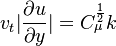
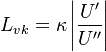
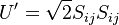
The following Bradshaw relation is used to express the relationship between $v_{t}$ and k and kL:

$v_{t}|\frac{\partial u}{\partial y}|=C_{\mu}^{\frac{1}{2}}{k}$

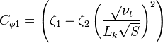
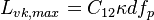
The parameters of the model are:

$C_{\phi 1}=\left(\zeta_{1}-\zeta_{2}\left(\frac{\sqrt{\nu_{t}}}{L_{k} \sqrt{S}}\right)^{2}\right)$

$C_{\phi 2}={\zeta_{3}}$

$L_{v k}=\kappa\left|\frac{U^{\prime}}{U^{\prime \prime}}\right|$

$U^{\prime}=\sqrt{2}{S_{ij}}{S_{ij}}$

$U^{\prime \prime}=\sqrt{\left(\frac{\partial^{2} u}{\partial x^{2}}+\frac{\partial^{2} u}{\partial y^{2}}+\frac{\partial^{2} u}{\partial z^{2}}\right)^{2}+\left(\frac{\partial^{2} v}{\partial x^{2}}+\frac{\partial^{2} v}{\partial y^{2}}+\frac{\partial^{2} v}{\partial z^{2}}\right)^{2}+\left(\frac{\partial^{2} w}{\partial x^{2}}+\frac{\partial^{2} w}{\partial y^{2}}+\frac{\partial^{2} w}{\partial z^{2}}\right)^{2}}$

$L_{v k , max}=C_{1 2}{\kappa}{d}{f_{p}}$

$L_{v k , min}=\frac{\sqrt{v_{t}}}{{C_{11}}{\sqrt{S}}}$

$f_{p}={min}{[max(\frac{P}{{\rho}{v_{t}}{S^{2}}} , 0.5) {,}{1.0}]}$

$f_{\phi}=\frac{1+C_{d1}{\epsilon}}{1+\epsilon^{4}}$

$\epsilon=\frac{d \sqrt{0.3\frac{{v_{t}}{S}}{a_{1}}}}{20v}$

$\zeta_{2}=\zeta_{1}-\frac{\zeta_{3}}{C_{\mu}^{\frac{3}{4}}}+\frac{\kappa^{2}\sigma}{ C_{\mu}^{\frac{1}{2}}}$

The model constants are:

$\zeta_{1}=1.5$

$\zeta_{2}=0.95$

$\zeta_{3}=0.16$

$\kappa=0.41$

$a_{1}=\sqrt{C_{\mu}}=0.3$

$C_{11}=10.0$

$C_{12}=1.3$

$C_{d1}=4.7$

$\sigma=0.6$

References

S. Shuai and R. K. Agarwal (2020), "A New Improved One-Equation Turbulence Model Based on k-kL Closure", AIAA Paper 2020-1075, January 2020.
K. S. Abdol-Hamid, J. R. Carlson, and C. L. Rumsey (2016), "Verification and Validation of the k-kL Turbulence Model in FUN3D and CFL3D Codes", AIAA 2016-3941, 2016.

Shuai-Agarwal turbulence Model

From CFD-Wiki

Introduction

Shuai – Agarwal One Equation k-kL Turbulence Model

References

Views

My wiki

wiki navigation

wiki search

wiki toolbox