CONVERGE FAQ

From CFD-Wiki

We hope you find the following FAQ helpful. For more information about many of the topics listed here, please review the CONVERGE documentation available on the CONVERGE Hub at hub.convergecfd.com/login (login required). In particular, the CONVERGE Manual, CONVERGE Studio Manual, Getting Started Guide, and training resources may be especially helpful. In addition, the example cases (each consisting of a surface geometry and input parameters) in CONVERGE Studio can provide a useful starting point for your own cases.

INSTALLING AND RUNNING CONVERGE

What are the hardware and software requirements for CONVERGE and CONVERGE Studio? How do I install CONVERGE or CONVERGE Studio?

Please refer to the Getting Started Guide for hardware and software requirements, installation instructions, and other related information.

Should I enable hyper-threading for my CONVERGE simulation?

CONVERGE, like other software packages that are designed to run on a large number of cores, does not run as efficiently when hyper-threading is enabled. This is true even when the number of processes in a simulation does not exceed the number of physical cores on the machine. For best performance, disable hyper-threading before running a CONVERGE simulation.

I see that CONVERGE offers various MPI implementations. Which one should I use?

Supported MPI packages are shipped with the CONVERGE installation package to reduce the likelihood of compatibility issues. If you have your own implementation of a supported MPI package, we recommend using that instead (refer to the Getting Started Guide for supported MPI versions). Otherwise, you can use any of the MPI packages shipped with the installation package.

Can CONVERGE run on GPUs?

CONVERGE 4 and earlier versions run exclusively on CPUs. Starting in CONVERGE 5, some simulations can utilize GPUs in conjunction with CPUs. GPU computation is a preliminary feature under active development. Refer to the CONVERGE Manual for information about the functionality that is currently supported on GPUs.

COMPUTATIONAL SPEED, MESH AND LOAD BALANCING

How does y+ AMR restriction work? Can I use this feature to ensure I have an acceptable mesh near the wall for the law-of-the-wall models?

CONVERGE has an option for y+ AMR restriction, which can restrict AMR cells close to the wall. You specify the target y+ and y+ ratio for this feature:

y+ target: If the y+ value of a cell near the specified boundary is less than the specified target, then at that time-step CONVERGE will remove one level of refinement from that cell. CONVERGE does not remove more than one level of refinement in a single time-step even if the resulting y+ value is still less than the target. It is important to ensure that the target y+ value is based on the turbulence model and corresponding wall model in your simulation.
y+ ratio: If the y+ value of a cell near the specified boundary is less than the product of the y+ target and the y+ ratio, then at that time-step CONVERGE will remove one level of refinement on all of the neighboring cells whose AMR level is equal to or greater than that of the original cell. CONVERGE does not remove more than one level of refinement in a single time-step even if the resulting y+ value is still less than the product of the y+ target and the y+ ratio.

You can use y+ AMR restriction to ensure that the mesh near the wall is appropriate for a law-of-the-wall model.

What is the maximum allowed level of AMR?

You can apply as many levels of AMR or fixed embedding as are required to resolve the flow physics of interest, although extremely small cells will limit the maximum time-step and increase the total wall-clock time.

Can I import my native CAD files directly into CONVERGE?

Yes, CONVERGE integrates the Spatial software package for direct import of most native CAD files. The Spatial import offers a resolution setting (coarse, medium or fine) for the interpolation of the CAD geometry to a triangulated surface in CONVERGE.

What is the best way to extract aero-volume from a CAD geometry?

The most direct approach is to use a CAD tool such as NX, SolidWorks, or whatever was used to create the surface. You can import the STL file (or use Spatial to read the CAD file) into CONVERGE Studio and delete the solid surfaces (if conjugate heat transfer is not part of the simulation). A more sophisticated workflow is required when the geometry is complex and includes minute details such as nuts, bolts or holes that are not a part of the fluid/aero volume.

Does CONVERGE have cell-based load balancing?

CONVERGE partitions the domain on a cell-by-cell basis. Cell-based load balancing can balance the computational load more equally for a large number of cores.

How are paired cells shown in 3D post-processing of CONVERGE?

In CONVERGE, the paired cells are shown as merged.

Can CONVERGE automatically improve the quality of the mesh in tight gaps?

CONVERGE offers a proximity-based type of AMR. This refines the mesh in tight gaps such as those in rotating machinery.

What is an inlaid mesh?

CONVERGE can solve cells that are constructed and inlaid within the octree cells. These are referred to as inlaid cells. Inlaid cells have a prescribed shape, size, and orientation. They can be used, for example, for boundary layer meshes or spray-aligned conical meshes. This feature allows the import of any grid to be used in conjunction with the typical CONVERGE Cartesian grid. You can also construct inlaid meshes in CONVERGE Studio. Note that inlaid meshes do not currently support AMR or fixed embedding.

Is the inlaid mesh automatically created at the start of simulation or during pre-processing?

Inlaid meshes are created during pre-processing in CONVERGE Studio. The inlaid mesh is defined as part of the geometry, and it belongs to the surface file.

How do I set up an inlaid mesh with CONVERGE?

Most inlaid meshes are constructed in CONVERGE Studio. First, create the inlaid mesh in the Geometry module of CONVERGE Studio. Then, set up the correct boundary conditions for all surfaces belonging to the user-made mesh. CONVERGE Studio also offers the capability to import stationary meshes from other software packages in Plot3D format.

Can an inlaid mesh in CONVERGE be attached to a moving boundary?

Yes, an inlaid mesh can be attached to a moving boundary or can interact with a moving boundary.

Can CONVERGE automatically match the cell sizes on a Cartesian-inlaid mesh interface?

CONVERGE offers an inlaid mesh neighbor type of AMR. This AMR type refines the mesh on the Cartesian side based on the cell size discrepancy between neighboring cells on either side of the INTERFACE boundary separating the inlaid and the Cartesian mesh.

How would having inlaid cells in my domain affect the load balancing in CONVERGE?

Inlaid cells are treated the same as Cartesian cells when it comes to load balancing. This means that regardless of how fine the inlaid mesh is, the load balancing will be as efficient as it would be without the inlaid cells. For reasons other than load balancing, a simulation with an inlaid mesh can be slightly slower than a similar case without the inlaid mesh, but this is not related to the load balancing. On the other hand, the inlaid mesh case may be faster if the inlaid mesh allows for a lower cell count.

How can I find more information about inlaid mesh and boundary layer mesh feature?

More information can be found in CONVERGE Manual. For additional assistance, please contact the Convergent Science Applications team [support@convergecfd.com (US), supportEU@convergecfd.com (EU), or support.in@convergecfd.com (India)].

My simulation runs slowly. How can I identify the cause?

A simulation might run slowly for a variety of reasons. First, look at the log file (or at time.out) to see what is limiting the time-step. If output_control > log_level = 3 in inputs.in, CONVERGE records in the log file and in time.out the time spent on each major routine (combustion, spray, load balancing, moving grids, etc.). These data can shed some light on the slowdown. Some common causes for a slow simulation are: too many parcels in a spray simulation, a large chemical mechanism in a combustion simulation, or a misconfigured cluster interconnect. CONVERGE almost always load balances well. You can review cell_count_ranks.out to understand and determine how to improve the load balancing.

The time-step in my simulation is limited by max_cfl_u. How can I accelerate my simulation?

When the variable time-stepping algorithm is used, CONVERGE controls the time-step by the user-specified CFL numbers (among other limiting criteria). When the convective CFL number limits the time-step, it may be due to small cell sizes or high flow velocities. You can use a region- and temporal-based CFL number to increase the time-step when important events are not occurring. For example, set temporal_control > max_cfl_u = 1 in inputs.in during combustion and increase it during the exhaust phase. Refer to the SI8 engine PFI SAGE example case (in CONVERGE Studio, go to File > Load example case) to see a demonstration of this technique. Turning off embeddings during less important times of the simulation (or in less important parts of the domain) may also help alleviate this restriction.

How can I speed up my multiple-cycle engine simulations?

CONVERGE features such as skip species, region- and temporal-based convective CFL number, and region- and temporal-based AMR can speed up multi-cycle engine simulations. The SI8 engine head CHT steady RANS example case includes these features.

My simulation slows down significantly when spray starts. What should I do?

A slowdown when the spray starts is expected, but there are some steps to take if you are concerned. First, check if the total number of injected parcels (num_parcels_per_nozzle) is set based on the recommended criterion for your grid size. Note that the specified number of parcels in spray.in is for a single nozzle, while the injected mass is for the entire injector. If you dramatically reduce the number of parcels, you should check how sensitive the predictions are relative to the injected number of parcels. If collision is turned on, verify that multiple nozzles do not reside in a single cell.

My turbomachinery simulation time-step is limited by dt_move. How can I make this simulation run faster?

A time-step limited by dt_move is a typical bottleneck in high speed turbo-machinery simulations. This time-step limit was put in place primarily for stability reasons. There are two options to try to get around this bottleneck and speed up your simulation: increase the cell sizes at the moving boundaries or relax the dt_move constraint. Note that either of these workarounds can affect the solution accuracy and stability.

The swept cell volume of any moving boundary is limited to a portion of cell in a single time-step. The default value in CONVERGE is 0.5 (i.e., in a single time-step, the moving boundary cannot sweep more that 50% of the smallest cut-cell volume). You can use values greater than 1.0, although higher values might affect solution stability or accuracy. To change this value in CONVERGE Studio 2.4+, go to Simulation Parameters > Simulation time parameters > Moving boundary time-step multiple.

Will the triangle count in my CAD file affect my simulation’s runtime?

Yes, especially for cases with moving boundaries. CONVERGE generates the grid at each time-step, and there is a computational cost in trimming Cartesian fluid cells. If a geometry contains an unnecessarily high triangulation, we recommend coarsening the surface to reduce the number of triangles while retaining the surface features. CONVERGE Studio contains a coarsening tool.

Think of it this way: a rectangle can be defined by two triangles. Alternatively, a poor CAD algorithm can define a rectangle of the same area by 1 million small triangles. This huge triangle addition can slow down simulations. For typical engine geometries, keep the triangle count around 0.3 to 0.5 million. In CONVERGE, the load balancing is based on cells. This means that, regardless of embed levels set for fixed embeddings and AMR, the solver can almost perfectly distribute the cells between the cores. The solver will automatically redo the load balancing, when the ratio of max cell in a rank to average cells per rank exceeds the simulation_control > imbalance_factor in inputs.in. CONVERGE rarely load balances poorly.

What is the optimum number of cells/processor for a typical ICE simulation?

Depending on the hardware (cluster and interconnect), you can efficiently run with fewer than 1500 cells per core.

How often does CONVERGE do load balancing?

In CONVERGE, the solver will automatically redo the load balancing when the ratio of the maximum number of cells in a rank to the average number of cells per rank exceeds the simulation_control > imbalance_factor that you specify in inputs.in.

OUTPUTS AND POST-PROCESSING

What are the new options for post-processing in CONVERGE?

CONVERGE 3.1 and later versions offer in-situ post-processing with ParaView Catalyst. CONVERGE reads and executes ParaView scripts at runtime, enabling the output of images and data while the simulation is running. ParaView Catalyst also allows you to post-process in parallel if the solver is being run on multiple cores. This feature may be useful for very large geometries or for design engineers simulating the same machine with different design variations.

How do I predict the ammonia uniformity index before SCR?

Ammonia uniformity is one of the major factors to look into during the SCR system design cycle. In CONVERGE, you can activate a feature to calculate the uniformity index based on selected cell variables, such as velocity, temperature, YNH3, and HNCO. You can specify the location, orientation, and region of the plane where the uniformity index is calculated.

Where do I see residuals in CONVERGE?

Starting in CONVERGE 4, residuals are written to the residuals.out file for all steady simulations. CONVERGE does not always use residuals to determine convergence. Instead, it uses a steady-state monitor approach where key quantities are monitored and criteria must be met for the case to become steady. The monitored quantities can be residuals and/or simulation variables, depending on the case.

How can I know at what time a restart file has been written? And how do I know if the file has been written properly?

In a terminal, type the following command to obtain the time at which a restart file was written: h5dump -a TIME_STEP <restart file name> If the above command does not work, the file may be corrupt. For legacy CONVERGE versions (2.3/2.4), the first line of the restart file includes the time, so you need to use a different command. To obtain the first line of the restart file, enter head -1 <restart file name> To check if the file has been written properly, type: tail -1 <restart file name>

Can a map file from an older version of CONVERGE be used for newer versions?

The map files for CONVERGE 3.1 and later versions are interchangeable. Map files for CONVERGE 3.0 can be used to run simulations with CONVERGE 3.1, but they must be converted to a different format to run simulations with CONVERGE 4+. Map files for CONVERGE 2.4 and older must be converted to a different format to run simulations with CONVERGE 3.0+.

If you need help converting a map file from CONVERGE 3.0 or earlier to run a simulation with a newer CONVERGE version, contact the Convergent Science Applications team [support@convergecfd.com (US), supportEU@convergecfd.com (EU), or support.in@convergecfd.com (India)].

Can Tecplot and ParaView directly read CONVERGE post output files?

Yes. Tecplot and ParaView can natively read the CONVERGE *.h5 post files from CONVERGE 3.0.8+.

How can I see how long CONVERGE spends on different processes (e.g., spray, combustion, and load balancing)?

In CONVERGE Studio, go to Simulation Parameters > Run parameters > Misc and set the Screen print level to Verbose or More verbose. Upon running the case you will see the below output in the log file either after every iteration (more verbose screen output) or at the end of simulation (verbose screen output) :

Time for ncyc 41 = 3.89 seconds

load balance = 0.00 seconds (0.00%)

solving transport equations = 3.37 seconds (86.50%)

move surface and update grid = 0.01 seconds (0.16%)

Combustion = 0.00 seconds (0.00%)

spray = 0.06 seconds (1.60%)

writing output files = 0.27 seconds (6.89%)

I ran two simulations with identical settings except that one simulation was initialized via mapping. Why are the results from these two simulations not the same?

The mapping data file does not save grid information and thus CONVERGE does not map data into the same cells. Instead, in a simulation with mapping, CONVERGE initializes each cell with data from the nearest point in the mapping data file. This process may result in some data smearing (i.e., several cells in the new simulation may be initialized with data from the same point in the map file). In addition, the AMR resolution from the old grid is not carried over to the new simulation. These differences are the reasons that the results are not identical.

What CONVERGE quantity can be compared against measured mass flow rate data at the intake port?

CONVERGE writes mass flow at the valves to regions_flow.out. CONVERGE writes mass flow rates from the inflow and outflow boundaries to mass_avg_flow.out and area_avg_flow.out.

How can I check the status of my simulation?

In the time.out file, check the wall time per time-step, which tells you how much time is being spent at each time-step or cycle. This quantity can give you an idea of whether your simulation is slowing down. You can also see if there are any recoveries in the simulation and what is causing the recoveries. The time.out file also contains the time-step size, what is limiting the time-step, and the values of the CFL numbers at each time-step.

Additionally, there is a log file written with each CONVERGE simulation which contains a lot of information. Depending on the verbosity level specified in inputs.in (output_control > log_level), the amount of information in this file will vary.

The NOx emissions in emissions.out and species_mass.out are not identical. What is the difference between these quantities?

The NOx emissions in emissions.out are from the extended Zel’dovich mechanism, which is hard-coded in CONVERGE. The calculated NO mass is multiplied by a factor of 1.533 to output NOx mass. This output is available even if you are not solving detailed chemistry. If you are using the SAGE detailed chemistry solver and if the chemical mechanism includes NOx species and reactions, then those species masses are recorded in species_mass.out. The NOx mass calculated using SAGE might not match exactly with that calculated using the extended Zel’dovich mechanism. In the passive NOx model, radicals [O] and [OH] can be assumed to be at equilibrium, while species NOx does not make such an assumption. This assumption in the passive NOx model is valid only at high temperatures (T > 2200 K). Quantities solved outside of this requirement might be responsible for the different NOx emissions data.

For 1DCHT cases, how can I view the surface temperature in a post-processor?

The bound_temp variable in post.in will give the surface temperature.

How can I obtain surface-averaged data on individual boundaries?

In CONVERGE Studio, go to Case Setup > Output/Post-Processing > Output files > Output generation and select Generate WALL boundary-averaged output. This option will generate a series of files named bound*-wall.out.

What is the difference between monitor points and super-cycle monitor points?

Monitor points are locations in the domain at which CONVERGE collects data during the simulation. The general monitor point option (monitor_points.in or Case Setup > Output/Post-Processing > Monitor points) allows you to place points throughout the domain and to select from a variety of variables to be monitored at those locations. CONVERGE writes monitor point data at each time-step.

Super-cycle monitor points (supercycle.in or Case Setup > Physical Models > Super-cycle modeling) provide temperature data from specific locations within the solid domain. CONVERGE writes super-cycle monitor point data at each super-cycle.

How can I output the prescribed heat transfer coefficient to the post*.out files?

Include bound_htc in post.in (Case Setup > Output/Post-Processing > Post variable selection).

COMBUSTION AND EMISSIONS

How can I determine the type of flame I should expect (i.e., premixed or non-premixed) for my applications using CONVERGE?

CONVERGE provides a post-processing variable called flame_index in post.in. It is a dot product of the fuel mass fraction and oxidizer mass fraction. If flame_index = -1, then the flame is non-premixed. If flame_index = 1, then the flame is premixed.

What is the thickened flame model in CONVERGE used for?

One of the challenges of obtaining accurate combustion simulations with laminar detailed chemistry (SAGE) and large eddy simulations (LES) is that the mesh should be refined sufficiently to resolve the flame thickness with at least a few cells. This can be a challenge for thin flames at high pressure. The thickened flame model (TFM) artificially thickens the flame by adding diffusivity and slowing the reaction rate. By increasing the diffusivity and reducing the reaction rate consistently, the flame speed is unchanged but the flame thickness is increased. TFM currently works with premixed or partially premixed gaseous fuels.

Where do I go in CONVERGE Studio to set up and generate an FGM table?

FGM table generation setup is activated in Chemistry > Chemistry Configuration > Table Generation: FGM. Once you have activated FGM table generation, go to Chemistry Setup > FGM Table Generation > FGM table generation to configure the fgm.in file. For more information about the FGM table, refer to the CONVERGE Manual.

When reducing a large mechanism typical of a gas turbine simulation, what physical parameters does CONVERGE maintain so that the reduced mechanism still emulates the original large mechanism?

In addition to ignition delay targets (simulated using 0D simulations), you can also ensure that the laminar flamespeed (simulated using 1D simulations) for the reduced mechanism is maintained within reasonable tolerances of the original mechanism.

The cells in my LES are not fine enough to resolve the laminar flame thickness. Is there a way to improve the results of my simulation?

In most large eddy simulations (LES) of premixed flames, the cells are not fine enough to resolve the laminar flame thickness. You can couple the SAGE detailed chemical kinetics solver with a dynamic thickened flame model to increase the flame thickness.

There is burning in the intake port in my G-Equation simulation. Why?

The G-Equation combustion model is active when the G_EQN passive is greater than or equal to zero. Thus, the entire simulation domain and the INFLOW and OUTFLOW masses must be set to a negative G value to avoid initializing flames from unintended locations. Refer to the SI8 engine premix G-Equation example case (in CONVERGE Studio, go to File > Load example case) for example settings.

There is burning in the intake port during the second cycle of my G-Equation simulation. The first cycle did not have this problem. Why is there burning in the second cycle?

Before the fresh unburned mixture enters the cylinder at the start of the second cycle, the entire simulation domain should be reinitialized with a negative value of G. To set up this option in CONVERGE Studio, go to Case Setup > Physical Models > Combustion modeling > Models (G-Equation) > Additional… > Initial G-value and select the Use file option. Refer to the SI8 engine premix G-Equation example case for an example of this setup (in CONVERGE Studio, go to File > Load example case).

Should I use temperature AMR in a G-Equation combustion simulation?

In simulations with the SAGE detailed chemistry solver, temperature AMR is used to resolve the flame front so that the flame propagation speeds (and thus the fuel burn rates) are correct. However, in the G-Equation model, the flame speeds are determined from a flamespeed correlation and so we recommend NOT activating temperature AMR. This will reduce the total cell count and allow the simulation to run faster. Note that CONVERGE does not prohibit the use of temperature AMR in a G-Equation simulation.

What laminar and turbulent flamespeeds are used in SAGE?

Unlike many simplified combustion models, the SAGE detailed chemistry solver does not calculate laminar and turbulent flamespeeds directly. When using SAGE for calculating premixed combustion, the turbulent flamespeed is the result of the chemical reaction rates (from the mechanism file, e.g., mech.dat) and the enhanced mixing from the turbulence model. Even though a flamespeeds are not directly calculated, the resulting turbulent flamespeed from the chemistry and turbulence model is St=Sl*(Dt/D)^0.5 and Sl is proportional to (reaction rate*D)^0.5. Again, the laminar flamespeed, Sl, and turbulent flamespeed, St, is not explicitly calculated in the SAGE approach.

How can I have CONVERGE write out laminar and turbulent flamespeeds in my SAGE simulation?

You can use the flamespeed correlations in the G-Equation combustion model. When you set up your simulation in CONVERGE Studio, go to Case Setup > Output/Post-Processing > Post variable selection > Cells and select Laminar Flame Speed and Turbulent Flame Speed. You must also select the desired correlations in Case Setup > Physical Models > Combustion modeling. Note that these calculated flamespeeds are not used in the SAGE calculations and give only an approximation of the flamespeeds that result from the SAGE solver.

My high-EGR case does not burn well with the same chemical kinetics mechanism that gave me good predictions for no- or low-EGR cases. What should I do?

This is a limitation of the mechanism. It is likely that the mechanism was not validated against ignition delay and laminar flamespeed data under high-EGR conditions. If such data are available, CONVERGE contains a mechanism tuning tool that can change the reaction rate coefficients to match the high-EGR data. See the CONVERGE Manual for more details about this feature.

What parameters are available to increase or decrease the burn rates in a SAGE simulation?

We recommend reviewing the grid and boundary condition settings for accuracy before trying to tune the reaction rates. The Reaction multiplier option can be used to increase or decrease fuel burn rates (in CONVERGE Studio, go to Case Setup > Physical Models > Combustion modeling > Models (SAGE) > SAGE Parameters). The turbulent Schmidt number can be reduced to enhance mixing and thereby increase burn rates, or it can be increased to slow mixing and thereby reduce burn rates (go to Case Setup > Physical Models > Turbulence modeling > Prandtl/Schmidt number/Viscosity).

The lower heating value (LHV) of the fuel used in the experiments is different from the fuel surrogate used in the simulation. How can I correct this?

In CONVERGE, you can specify LHVs for individual species. The data in the thermodynamic data file (e.g., therm.dat) will be adjusted to recover the user-specified LHV. To set up this option in CONVERGE Studio, go to Case Setup > Materials > Gas simulation > Thermodynamic files and check Lower heating value. Open the accompanying dialog box to specify the species-specific LHVs.

How can I calibrate the ignition delay in the Shell ignition model?

In CONVERGE Studio, go to Case Setup > Physical Models > Combustion modeling > Models (CTC/Shell) and adjust the Ignition delay constant (af04). Increasing this value will reduce the ignition delay.

Can the RIF model be used to simulate premixed combustion in CONVERGE?

No. CONVERGE’s RIF model can be used only for non-premixed combustion.

Does the RIF model require an autoignition model in order to simulate diesel combustion?

No. CONVERGE’s RIF model uses the provided chemical kinetics mechanism to capture ignition delay.

Does CONVERGE use pre-compiled flamelet libraries (lookup tables) or does CONVERGE solve the kinetics in the mixture fraction space on the fly?

For the FGM model, CONVERGE uses pre-compiled flamelet libraries. For the RIF model, CONVERGE solves the kinetics in the mixture fraction space on the fly.

Does the RIF model in CONVERGE support unsteady and multiple flamelets?

Yes.

Can I use the same mechanism for the SAGE detailed chemistry solver and the RIF model?

Yes, but note that you cannot run both SAGE and RIF in a single simulation.

What advantage do the simplified combustion models have compared to the SAGE detailed chemistry solver?

The simplified combustion models are generally faster than SAGE.

Do the phenomenological, PM, and PSM soot models work with the RIF combustion model?

Yes.

Which species and reactions are considered in the CTC model?

The CTC model considers CO, H2, CO2, O2, H2O, N2, and the fuel. The Combustion Modeling chapter of the CONVERGE Manual describes the reactions in the CTC model.

Which parameters should I change to calibrate the CTC model?

Increasing the Turbulence time-scale constant will decrease the rate of combustion. You can also adjust the Chemical time-scale constant. To change these parameters in CONVERGE Studio, go to Case Setup > Physical Models > Combustion modeling > Models (CTC/Shell).

How can I avoid having my soot values oscillate close to EVO?

You can tighten the passive tolerance. More generally, however, we recommend ending combustion before EVO.

Can I predict engine knock using the G-Equation model?

Yes, you can predict engine knock via G-Equation as long as you are using a version of the G-Equation model that includes the SAGE detailed chemistry solver outside of the flame front (the G = 0 surface). In CONVERGE Studio, go to Case Setup > Physical Models > Combustion modeling > Models (G-Equation) and select one of the options that includes SAGE outside of the flame front.

When using ECFM3Z, how can I generate my own TKI tables?

This can be done using the Table Generation: TKI option in CONVERGE Studio’s Chemistry module. Refer to the Constant pressure ignition delay table generation example case (in CONVERGE Studio’s Chemistry module, go to File > Load example case).

Can I use ECFM+TKI for knock simulations?

Yes, ECFM+TKI is available in CONVERGE and can be used to predict engine knock.

Can I use ECFM or ECFM3Z for GDI/PFI engines?

Both models can be used for GDI/PFI engine simulations. However, we do recommend using ECFM instead of ECFM3Z if the mixing time is short or the grid resolution is not fine enough.

How can I convert a map.out file from a SAGE simulation for use with an ECFM simulation?

Please contact the Convergent Science Applications team [support@convergecfd.com (US), supportEU@convergecfd.com (EU), or support.in@convergecfd.com (India)] to obtain a script for this conversion.

How do I account for the fuel’s cetane number?

When using the SAGE detailed chemistry solver, you can use a fuel blend that has the same cetane number as the fuel used in the experiments. It is important to ensure that all of the surrogate fuel species are available in your chemical kinetics mechanism.

When using the CTC/Shell model for diesel combustion, one of the reaction rates in the shell model can be made a function of the cetane number via a user-defined function. For details, please see the following paper:

Ayoub, N. and Reitz, R., "Multidimensional Modeling of Fuel Composition Effects on Combustion and Cold-Starting in Diesel Engines," SAE Technical Paper 952425, 1995, doi:10.4271/952425

Can CONVERGE tune kinetic mechanisms to match ignition delay and laminar flamespeed data?

Yes. The mechanism tuning tool can be used to optimize mechanisms to match ignition delay and laminar flamespeed data for multiple operating points. Please see the CONVERGE Manual for more details.

CHEMISTRY TOOLS

What can I do with CONVERGE’s chemistry tools?

The chemistry tools allow you to study reacting systems, manipulate mechanisms, and generate data tables needed for some simulations. Examples: The chemistry tools allow you to study reacting systems, manipulate mechanisms, and generate data tables needed for some simulations. Examples:

Blending surrogate fuels to match real fuel properties

Reducing, tuning, and merging kinetic mechanisms to extend or alter their usage

Calculating ignition delay (ID) and laminar flamespeed of combustible mixtures to examine flammability, compare different fuel and oxidizer combinations, or evaluate kinetic mechanisms
Creating laminar flamespeed tables and kinetics of ignition tables (TKI) for G-Equation and Extended Coherent Flamelet Model (ECFM) combustion models
Creating ID tables for 3-Zone ECFM (ECFM3Z) combustion model
Creating Flamelet Generated Manifold (FGM) tables for FGM combustion model

Do I need a separate license to run CONVERGE’s chemistry tools?

Running chemistry tools requires a valid CONVERGE license but it does not count as a license in use.

Can I run 0D and 1D cases in parallel?

Yes, these cases can be distributed to run on different processors. However, a single case cannot be run on multiple processors.

What can I calculate with 0D tools?

Zero-dimensional tools can be used to calculate the following quantities:

Ignition delay or equilibrium conditions of a system
Conditions in a homogeneous charge compression ignition (HCCI) engine
Research octane number (RON) and motor octane number (MON) of a given fuel
Ignition limits in flowing or well-mixed systems
Ignition delay targets for mechanism tuning
Speciation (calculated from flow reactor and shock tube equivalent simulations)

What are some aspects of the 0D reactor modeled in CONVERGE?

Single cell calculations without CFD boundary conditions

Runs to a user-specified end time: Equilibrium, autoignition, specified time
Mimics various processes
- For example, constant V, constant P and h
Can account for mass flow rates
- Well-stirred reactor and plug flow reactor
Can account for volume change
Can account for wall heat transfer

Can the chemical equilibrium (CEQ) conditions be calculated via CONVERGE’s chemistry tools?

Yes, 0D chemistry tools can be used to quickly find the equilibrium conditions of a reacting system. CEQ can be found under two thermodynamic conditions: (1) constant enthalpy and constant pressure or (2) constant temperature and constant pressure.

What ignition delay (ID) definitions does CONVERGE use?

Single ignition delay
- The time (t) to raise the mixture temperature by 400 K
Double ignition delay
- The first ignition delay (t1) is the time at which the first derivative of temperature with respect to time is at its maximum
- The second ignition delay (t) is the time to raise the mixture temperature by 400 K

What does the 0D engine RON/MON estimator do?

The RON/MON estimator determines the octane numbers of a given fuel composition per ASTMD2699 and D2700 standards.

For a given fuel, this tool finds the lowest compression ratio (critical compression ratio [CCR]) at which the mixture autoignites.
This tool compares the CCR to the CCR values of primary reference fuels (PRF) to determine the octane rating.

Can I use chemistry tools to explore the flammability limits of a mixture?

Yes, you can use the 0D well-stirred reactor model to explore combustion and flammability limits in turbulent, well-mixed systems.

What quantities can I calculate with 1D tools?

You can use one-dimensional simulations to accomplish a variety of processes:

Assess burning (laminar flamespeed) at certain mixture conditions
Evaluate the performance of a reaction mechanism
Generate laminar flamespeed targets for mechanism tuning
Develop laminar flamespeed tables necessary for some applications (TLF for ECFM, TLF for G-Equation, etc.)
Complete laminar counterflow calculations, which determine the temperature and species between two inlet streams

Can I use chemistry tools to create laminar flamespeed tables?

Yes, the 1D solver can be used to create laminar flamespeed tables that can be used by many combustion models, including the G-Equation model, the Extended Coherent Flamelet Model (ECFM), the thickened flame model (TFM), and the Flamelet Generated Manifold (FGM) model.

The lookup table can store laminar flamespeeds as a function of unburned temperature, pressure, equivalence ratio, EGR fraction (constant by default or tracked as passives if spatial and/or temporal variation are needed, unburned fuel species (traced as passives).

CONVERGE Studio can generate input files that can be used to generate flamespeed tables.

Can CONVERGE reduce kinetic mechanisms while conforming to ignition delay and laminar flamespeed targets?

Yes. The mechanism reduction tool can be used to reduce mechanisms while conforming to ignition delay and laminar flamespeed targets.

Can CONVERGE tune kinetic mechanisms to match ignition delay and laminar flamespeed data?

Yes. The mechanism tuning tool can be used to optimize mechanisms to match ignition delay and laminar flamespeed data for multiple operating points.

Can I use a chemistry tool to merge two chemical mechanisms?

Yes. The mechanism merge tool can combine two reaction mechanisms to:

Develop multi-component surrogate mechanisms (e.g., adding isooctane reactions to an n-heptane mechanism to develop a PRF mechanism)
Add PAH or NOx chemistry to a fuel mechanism to add emissions prediction capability
Add additional reaction pathways (e.g., adding more fuel reactions or additional pathways to secondary species to a skeletal mechanism)

It is important to validate the merged mechanism against available laminar flamespeed, species, and other data.

What is the surrogate blender?

CONVERGE Studio’s surrogate blender creates a multi-component fuel surrogate with specified physical properties. Since fuels consist of a mixture of several individual components, simulating a fuel as a single component can lead to errors. You can simulate fuels as multi-component surrogates whose properties (e.g., derived cetane number, molecular weight, H/C ratio) approximate those of the target fuel.

LAGRANGIAN PARCEL MODELING

What film splash models are available for aftertreatment simulations?

CONVERGE offers the O’Rourke, Kuhnke, and Bai-Gosman film splash models. For aftertreatment simulations, the Kuhnke model is commonly used. By altering model parameters like the rebound Weber number and non-dimensional critical wall temperature, you can alter model parameters to correlate the model to experimental results. The Wruck heat transfer model is also available to account for the Leidenfrost effect.

Can CONVERGE write out important spray statistics such as SMD or mass flux from a Lagrangian spray simulation?

CONVERGE contains a built-in Phase Doppler Particle Analyzer (PDPA). CONVERGE will track particles passing through user-defined PDPA points and compute relevant statistics (Sauter mean diameter, velocity components, mass flux, etc.) for each PDPA monitor point.

I am simulating a symmetric multi-hole injector, but the spray penetration patterns from each nozzle are not identical. The spray plumes aligned with the grid seem to penetrate more than the non-aligned plumes. Why?

Depending on the flowfield, there are cases in which the spray plumes will not be identical even though the spray nozzles are symmetric. In other cases, where the spray is dominant and the plumes are expected to be similar, this phenomenon is caused by numerical viscosity associated with large computational cell sizes. A spray injected along the diagonal of a cubic cell is subjected to more numerical viscosity than a spray aligned with the edges of the cells. This effect diminishes as the cells are refined. For more information, please refer to the Convergent Science white paper on numerical viscosity. In CONVERGE, you can specify a conical inlaid mesh along the axis of all nozzles. The inlaid mesh will minimize the uneven effects of numerical viscosity and produce more uniform plumes. Note that in some cases the non-uniformity of the flow will cause non-identical spray penetration for each of the plumes. This is a physical effect rather than a numerical one.

My spray simulation runs slowly due to significant wall film formation. Is there a way to increase the simulation speed?

CONVERGE offers a parcel consolidation option in which parcels at boundary cells are combined to reduce simulation time. This option is appropriate for simulations that run slowly because they have so many parcels at the wall.

Can I run VOF one-way coupling on CONVERGE 3.0 with a VOF map file that was created with an older version of CONVERGE?

Yes, CONVERGE can load a vof_spray.dat file that was written by an older version of CONVERGE as long as the Injector IDs and Nozzle IDs in the older files match the injector names and nozzle names in the parcel_introduction.in file.

What are the benefits of using inlaid mesh in spray simulations, and what are the limitations?

CONVERGE simulations can include cells that are not part of the global Cartesian cut-cell mesh. These cells, which can be of arbitrary size, shape, and orientation, are referred to as inlaid cells. Inlaid cells can be used, for example, to create spray-aligned conical meshes or boundary layer meshes. A spray-aligned mesh will lower the numerical diffusion associated with misalignment of the Cartesian grid with the nozzle axis. The spray-aligned inlaid mesh is especially useful for multi-nozzle sprays and can preserve consistency across individual nozzles and predict a more accurate liquid and vapor penetration length. A boundary layer mesh can resolve the boundary layer structure with many fewer cells than a Cartesian cut-cell mesh would require. Currently, AMR is not permitted in inlaid cells. The inlaid mesh is defined as part of the geometry and it belongs to the surface file; therefore, the inlaid mesh cannot intersect with any other boundaries of the geometry.

Does CONVERGE provide any models for mimicking flash boiling sprays?

When modeling drop evaporation, CONVERGE can apply a flash boiling model. CONVERGE can also reduce the drop size based on flash boiling. This feature can be activated in CONVERGE Studio via Case Setup > Parcels configuration > Liquid parcels > Click Edit to open the [LiqParcel#] editor > Evaporation > Flash boiling.

Must I increase the number of spray parcels when I refine the grid?

Yes. If the cell size is reduced and the number of parcels stays constant, then the amount of liquid in a cell increases, which tends to artificially reduce the drag on the droplet. Each time the cell is refined one level (e.g., when amr_groups > amr_group > amr_* > embed_scale in amr.in changes from 2 to 3), you should increase the number of parcels injected by at least a factor of 4 (8 is even better but can get very computationally expensive for fine meshes). Please consult the following publication for more details:

Senecal, P.K., Pomraning, E., Richards, K.J., and Som, S., “Grid-Convergent Spray Models for Internal Combustion Engine CFD Simulations,” Proceedings of the ASME 2012 Internal Combustion Engine Division Fall Technical Conference, ICEF2012-92043, Vancouver, BC, Canada, September 23-26, 2012. DOI:10.1115/ICEF2012-92043

Which pressure should be used to calculate parcel velocities in the spray rate calculator?

In order to calculate the parcel velocities that come out of the nozzle hole, we recommend using the difference between the injector sack pressure and the back pressure (cylinder pressure).

In the Kelvin-Helmholtz model, is the shed mass constant applied only to parent parcels or is it applied to any droplets subjected to a breakup event?

The shed mass constant (in CONVERGE Studio, go to Case Setup > Physical Models > Parcel breakup) is applied to all droplets in the domain that are undergoing KH breakup.

Does the Kelvin-Helmholtz model act only on parent parcels or does it also act on the first generation of child droplets (i.e., the droplets derived from the primary breakup)?

The KH model acts on all drops.

Is it correct to apply the Kelvin-Helmholtz model to the breakup of child droplets (i.e., not parent parcels), when the KH theory refers only to the disintegration of liquid jets (i.e., parent parcels)?

The KH model assumes that the fastest growing surface wave is much smaller in magnitude than the surface on which it grows, and thus it does not matter if it grows on a liquid sheet, a ligament, or a spherical drop.

How are primary and secondary breakup simulated in the modified KH-RT model?

Primary breakup is simulated via the KH model. For secondary breakup, the KH and RT models compete against one another.

In the KH-RT model, which parameters can be adjusted to change the drop size?

You can adjust several KH and RT parameters, but we recommend two of them as a starting point. In CONVERGE Studio, go to Case Setup > Physical Models > Parcel breakup. The parameters below are in that dialog box.

RT model size constant (rt > size_const): Reduce this value to reduce the drop size.
KH model breakup time constant (kh > time_const): Reduce this value to make drop breakup occur more quickly and to reduce the drop size.

How are the blobs initialized when the injection drop distribution is based only on nozzle size and the discharge coefficient model uses a varying nozzle velocity coefficient?

CONVERGE dynamically calculates the velocity coefficient (Cv) based on the injection pressure at that time. CONVERGE then calculates the contraction coefficient (Ca) from Ca = Cd/Cv (Cd is user-specified).

Once Ca has been calculated, CONVERGE calculates the effective diameter (deff) and effective area (Aeff) of the blob according to the following relationships:

$D_{blob}=d_{eff}=\sqrt{C_a}*d_0$

$A_{eff}=C_a*A_0$

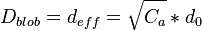
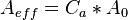
In the equations above, $d_0$ and $A_0$ are the nominal diameter and nominal area of the blob.

When should I use a spray-wall interaction model?

You should use a spray-wall interaction model whenever the spray impinges on a wall.

Are there any guidelines on the meshing requirements for spray-wall interaction models?

CONVERGE has no special meshing requirements for the spray-wall interaction models. You can use the typical grid recommendations.

Can a single liquid parcel species evaporate into multiple gas-phase species?

Yes, this can be done using composites, which are composed of multiple base species. To set up composites in CONVERGE Studio, go to Case Setup > Materials > Composite species. Please refer to the Engine sector diesel SAGE composite example case.

Can I use non-liquid parcels (e.g., solid or gas) in CONVERGE?

Yes, you can use liquid, solid and, starting in CONVERGE 5, gas parcels for various applications (e.g., liquid parcels for sprays, solid parcels for entrained dust, and gas parcels for high-speed jets).

AFTERTREATMENT AND UREA/SCR

To predict deposit formation, should I use the molten solid approach or detailed urea decomposition?

Because detailed decomposition of urea is as fast as molten solid decomposition in CONVERGE, we suggest using detailed decomposition and fixed flow to directly simulate the formation of species such as biuret, ammelide, and cyanuric acid (CYA).

Can I predict urea deposit mass and location in CONVERGE?

Yes. It’s recommended to use the deposit solidification model coupled with the urea detailed decomposition model to predict the deposit mass, composition and location in a urea/SCR system. With the help of acceleration schemes, like the fixed flow, the spray database, and the CHT supercycling, CONVERGE can simulate deposit growth over hours of experimental duration.

How can I accelerate my aftertreatment simulation to predict deposit formation over the course of hours?

For some continuous or pulsed spray simulations, the flow field may temporarily reach a pseudo steady-state. To reduce the total simulation time, CONVERGE offers a fixed flow option that freezes the flow field while still solving the spray. When the flow field is frozen, the spray is one-way coupled to the flow (i.e., the spray reacts to the flow but the flow does not react to the spray). This approach greatly extends the time-step (CFL number) so that 30 to 60 seconds of simulation time can be achieved in a single day. The newly implemented spray database, coupling with the fixed flow approach can further speed up the deposit simulations. The database approach would record spray parcels data when hitting on the walls and re-emit those recorded parcels during the emit cycles.

I am looking at NH3 uniformity of my urea/SCR. Do I need to use fixed flow?

Prior to CONVERGE 3.0.15, fixed flow was reserved for filming and deposit simulations, which require a long time to fully develop. Fixed flow is not eligible for NH3/HNCO uniformity studies since species in the flow domain would be fixed when fixed flow is turned on. However, in CONVERGE 3.0.15+, the species solver can be turned on when fixed flow is activated. This new feature allows uniformity studies to take full advantage of the fixed flow speedup.

Can I run catalyst surface chemistry simulation in CONVERGE?

Yes. CONVERGE supports region-based and boundary-based surface chemistry modeling, in which you can specify regions/boundaries in which surface chemistry will be solved and configure washcoat properties. CONVERGE also offers a new SPLIT surface chemistry solver to predict surface chemistry reactions from DETCHEM. Currently, CONVERGE offers surface chemistry example cases that cover SCR, DOC, LNT, and TWC.

Can I use the steady solver for my urea/SCR simulation?

Both the pseudo-transient steady solver and the under-relaxation steady (URS) solver are good for pressure drop predictions. URS performs better in terms of run speed and is recommended for urea/SCR system pressure drop simulations.

What is the urea deposit risk model, and how does it compare to the urea deposit solidification model?

The urea deposit risk model is a highly empirical approach that considers the conditions of the film (e.g., temperature, film height, HNCO concentration in gas near film surface) that promote urea deposit formation. The urea deposit risk model requires calibration to experimental data to be predictive. The deposit risk model can assess the risk levels of urea deposit formation in a urea/SCR system, while the deposit solidification model can quantitatively predict the deposit mass and composition over a long period of time.

Can CONVERGE model gasoline/diesel particulate filters (GPF/DPF)?

Yes. CONVERGE can predict the pressure drop and filtration efficiency during the soot loading process for both GPF and DPF. To speed up, a filter sector is modeled to represent the whole filter brick. The soot accumulation and ash accumulation effects can be studied as well in CONVERGE.

I am interested in TWC catalyst light off modeling. What models can I use?

The local thermal non-equilibrium model (LTNE) can be turned on for the light off simulation of TWC. The LTNE model enables gas and solid heat transfer in the TWC porous medium and solves the energy transport equation for gas and solid substrate separately.

EULERIAN MULTI-PHASE MODELING

Can CONVERGE apply its volume of fluid model for both compressible and incompressible fluids?

Yes. The VOF model in CONVERGE offers the Individual Species Solution (ISS) method and the Void Fraction Solution (VFS) method. The ISS, also known as compressible VOF, is good for compressible gases and compressible or incompressible liquids. The Void Fraction Solution method is good for incompressible gases and incompressible liquids.

In the VOF model, how does CONVERGE calculate the void fraction?

In the ISS method, i.e., compressible VOF, CONVERGE solves the individual species conservation equations and then calculates the void fraction from the cell mass fractions of liquid and vapor species. In the VFS method, or incompressible VOF, CONVERGE directly solves a transport equation for the void fraction.

Can CONVERGE predict the phase change of fluid due to flashing or cavitation?

Yes, the VOF model offers multiple cavitation models that can be used to predict the phase change of the fluid, including a homogeneous relaxation model and homogeneous mixture models.

Can Adaptive Mesh Refinement be used in a VOF simulation to reduce computation time?

Yes. When performing a VOF simulation, it is important to invoke Adaptive Mesh Refinement (AMR) on both void fraction and velocity to accurately simulate the interface between the liquid and the vapor. VOF models typically require fine resolution and thus small time-steps. Using AMR to add resolution where necessary can reduce cell count and computational time.

Can CONVERGE accurately capture the location of the interface between the liquid and the gas?

The use of AMR allows CONVERGE to locate the interface, but the high-resolution interface capturing (HRIC), flux-corrected transport (FCT), and piecewise linear interface calculation (PLIC) schemes greatly enhance the sharpness of the interface. Use HRIC or FCT with the ISS method and PLIC with the VFS method.

Can CONVERGE predict the atomization and evaporation of a liquid in a VOF simulation?

Predicting the atomization of the liquid in a VOF simulation requires (1) the Eulerian-Lagrangian Spray Atomization (ELSA) model, (2) the VOF one-way coupling approach, or (3) setting the grid size to be smaller than the size of the smallest droplets. The ELSA model automatically transitions Eulerian liquid to the Lagrangian parcel phase when the cell meets certain criteria. The VOF one-way coupling model initializes a Lagrangian parcel simulation using the data from a VOF simulation. In both cases, CONVERGE applies models for collision, drag, break-up, and evaporation to the Lagrangian parcels. The evaporation of a liquid in a VOF simulation can be predicted with the Lee boiling model. The Lee boiling model is available only for simulations using the individual species solution (ISS) method.

WALL HEAT TRANSFER

If I am interested in filming and urea deposit formation, should I use conjugate heat transfer for wall modeling?

Yes. Conjugate heat transfer (CHT) is usually used for simulations with filming and urea deposit formation. An accurate wall temperature prediction is crucial for filming simulations. Also, the urea decomposition by-products formation is rather sensitive to the film temperature, which requires a high-fidelity wall temperature prediction. We recommend super-cycling in conjunction with the CHT model to allow the walls to reach thermal equilibrium faster

How can I simulate thermal barrier coating using CONVERGE?

There are several ways to simulate thermal barrier coating (TBC) on a piston top. Here are a few options:

A full 3D CHT simulation, where the TBC is simulated as well as the rest of the piston. In this type of simulation, the thickness of the coating needs to be resolved, which means that there needs to be a sufficient number of cells across the thickness of the coating. This type of simulation is very expensive because it requires many cells and small time-steps.
A 3D CHT simulation plus contact resistance modeling, where the TBC is not simulated. In this type of simulation, the TBC is represented by a contact resistance on the surface of the piston and the rest of the piston is simulated. The contact resistance can be calculated based on the conductivity of the material used for the TBC and the thickness of the coating. The rest of the piston needs to be resolved. This type of simulation is more expensive than a gas-only internal combustion simulation but far less expensive than a full 3D CHT simulation.
A 1D CHT boundary condition, where the piston is not resolved and the TBC is represented by a 1D CHT boundary condition on the piston surface. This type of simulation is generally as expensive as a gas-only internal combustion simulation. There is some loss of accuracy because the heat transfer using the 1D CHT boundary condition is assumed to be only in one direction. In addition, some information about the internal temperature of the piston needs to be provided, which is not always known.

Can CONVERGE seal surfaces on an INTERFACE?

At this time, CONVERGE allows sealing on an INTERFACE that is NOT a flow-through INTERFACE.

What interpolation method does CONVERGE use for spatial boundary condition profiles?

CONVERGE does not interpolate for spatial boundary condition profiles. Instead, CONVERGE obtains information from the nearest data point.

When I run a CHT case, my case crashes and I see the following error: The surface has a non-interface triangle that is only connected to a single interface triangle. What is the problem?

This error is often related to an incorrect INTERFACE assignment. An edge can be shared by two triangles only if both triangles are non-interface or if both triangles are interface. CONVERGE does not allow an edge to be shared by one interface triangle and one non-interface triangle.

When I run a CHT case, my case crashes and I see the following error: Neighboring triangles are associated with different streams. What is the problem?

This error is often associated with an INTERFACE boundary. For an INTERFACE boundary, the surface normal of all triangles in that boundary must point toward the same region and that region must be consistent with the information in the boundary definition file (in CONVERGE Studio, go to Boundary Conditions > Boundary to set up this region). You may see the error specified above if a single surface normal points in the wrong direction.

I am comparing heat transfer coefficients (HTCs) from CONVERGE with HTCs from other codes and they do not match. Why?

In CONVERGE, the HTC is a local value based on the near-wall cell temperature, not a free-stream temperature. This HTC differs from an HTC that is based on a user-specified reference temperature, and it also differs from an HTC that could be estimated from a Nusselt number correlation. Because HTC definitions vary from code to code and because CONVERGE uses local HTC values that depend on the near-wall mesh, we recommend instead comparing flux.

Can we perform an all-in-one coolant/combustion/solid simulation?

Yes, CONVERGE can perform an all-in-one coolant/combustion/solid simulation with a multi-stream case setup (i.e., assigning the coolant, combustion gas, and solid to 3 different streams). In CONVERGE, a stream is a set of regions that share the same computational grid and the same phase. Connected streams are coupled to each other through INTERFACE boundaries. CONVERGE solves for each stream independently except for the coupled stream-to-stream INTERFACE, allowing for different numerical settings in each stream. CONVERGE will assign each stream to a specific transport group. Streams in the same transport group are solved in the same PISO or SIMPLE loop, and therefore must have the same time-step and the same solver setup. Streams in different transport groups (e.g., transient fluid and transient solid streams) can advance with disparate time scales, and the user can set up cross-stream synchronization to control how often the solutions for different transport groups are synchronized at the stream-to-stream interface.

Can I use super-cycling for predicting a steady-state temperature field in a non-engine case? If so, how do I set supercycle_stage_num and supercycle_stage_interval?

CONVERGE allows super-cycling in non-engine cases. As long as the temperature of the solid part can be approximated as a steady state, you can use super-cycling to obtain a steady-state solid temperature distribution faster than in a typical transient simulation. If the simulation has temporally periodic variation in its behavior (for example, as in an engine), supercycle_num_stages*supercycle_stage_interval must equal the cyclic period. For example, you may have a nozzle in a tunnel that is spraying water into the airflow for 1 minute in every 10 minutes. You can set supercycle_num_stages = 1 and supercycle_stage_interval = 10 minutes to obtain a steady-state temperature distribution in the solid tube wall through super-cycling. This configuration would average the heat transfer information for the full 10 minutes into one representative average and then perform the super-cycle calculation just once in every 10-minute period. Alternatively, you could set supercycle_num_stages = 5 and supercycle_stage_interval = 2. For this configuration, the average heat transfer information would be stored in 2-minute segments and CONVERGE would perform super-cycling 5 times in every 10-minute period. If the entire simulation is steady-state (both the fluid dynamics and solid portions), then there is no reason to use more than one stage for averaging the heat transfer information. In this case, set supercycle_num_stages = 1, and then choose the supercycle_stage_interval to be the window size for calculating the average heat transfer information used in super-cycling.

What is the convection temperature boundary condition?

In CONVERGE, you can set a convection boundary condition for either a solid or a fluid WALL boundary. In either case, the convection boundary condition prescribes the convection between the wall and the environment (note that the environment is not included in the computations).

OPTIMIZATION

How many simulations are typically required when optimizing an engine case in CONVERGE using the genetic algorithm utility CONGO?

We recommend 50-100 generations, which would be about 800 simulations, for an optimization including 5-10 parameters.

Is optimizing a mechanism using the mechtune capability similar to optimizing a CFD case?

It depends on which optimization method you choose when you run the mechanism tune (mechtune) utility. We recommend using NLopt, which is based on the open-source NLopt library and does not require the use of CONGO. If you choose a genetic algorithm with CONGO as the optimization method, the mechtune utility will create input files for CONGO. We recommend a minimum of 2000 generations for a mechanism tune case (~16,000 ignition delay/flamespeed simulations). See the following paper for a demonstration of this capability:

Mittal, A., Wijeyakulasuriya, S.D., Probst, D., Banerjee, S., Finney, C.E.A., Edwards, K.D., Willcox, M., and Naber, C., "Multi-Dimensional Computational Combustion of Highly Dilute, Premixed Spark-Ignited Opposed-Piston Gasoline Engine using Direct Chemistry with a New Primary Reference Fuel Mechanism," ASME 2017 Internal Combustion Engine Division Fall Technical Conference, ICEF2017-3618, Seattle, WA, United States, Oct 15–18, 2017. DOI: 10.1115/ICEF2017-3618

Is it possible to optimize geometry features in CONVERGE?

Yes, this capability is a strength of CONVERGE. Because CONVERGE creates the mesh at runtime, modifying the geometry in optimization is straightforward. The surface file can be parameterized using CAD or a number of third-party geometry-modifying software packages. More information is available from the following resources:

Pei, Y., Pal, P., Zhang, Y., Traver, M., Cleary, D., Futterer, C., Brenner, M., Probst, D., and Som, S., "CFD-Guided Combustion System Optimization of a Gasoline Range Fuel in a Heavy-Duty Compression Ignition Engine Using Automatic Piston Geometry Generation and a Supercomputer," SAE Paper 2019-01-0001. DOI: 10.4271/2019-01-0001
Automated Optimization Workflow for a Diesel Piston Bowl Using CAESES and CONVERGE CFD” webinar recording, available on the CAESES website.

How can machine learning be used to enhance optimization of CONVERGE cases?

Machine learning can be used to build an emulator for CFD using design of experiments data to characterize the design space. The machine learning emulator can then be used for optimization, sensitivity, and uncertainty quantification. Several papers have demonstrated the utility of this approach (including the two listed below). Please contact the Convergent Science Applications team [support@convergecfd.com (US), supportEU@convergecfd.com (EU), or support.in@convergecfd.com (India)] if you are interested in learning more.

Moiz, A.A., Pal, P., Probst, D., Pei, Y., Zhang, Y., Som, S., and Kodavasal, J., “A Machine Learning-Genetic Algorithm (ML-GA) Approach for Rapid Optimization Using High-Performance Computing,” SAE Paper 2018-01-0190. DOI:10.4271/2018-01-0190
Probst, D.M., Senecal, P.K., Qian, P.Z., Xu, M.X., and Leyde, B.P., "Optimization and Uncertainty Analysis of a Diesel Engine Operating Point using CFD," Proceedings of the ASME 2016 Internal Combustion Engine Division Fall Technical Conference, ICEF2016-9345, Greenville, SC, United States, Oct 9–12, 2016. DOI: 10.1115/ICEF2016-9345

Does CONVERGE / CONGO include machine learning capability for optimization?

CONVERGE 5 introduces a Machine Learning (ML) optimization tool. You can use the ML tool to configure a design of experiments, simulate points in the search space with CONVERGE, train an emulator to propose an optimum design, test the proposal with CONVERGE, and augment the training set iteratively until you have found the global optimum of your search space.

CONVERGE FAQ

From CFD-Wiki

Contents

INSTALLING AND RUNNING CONVERGE

What are the hardware and software requirements for CONVERGE and CONVERGE Studio? How do I install CONVERGE or CONVERGE Studio?

Should I enable hyper-threading for my CONVERGE simulation?

I see that CONVERGE offers various MPI implementations. Which one should I use?

Can CONVERGE run on GPUs?

COMPUTATIONAL SPEED, MESH AND LOAD BALANCING

How does y+ AMR restriction work? Can I use this feature to ensure I have an acceptable mesh near the wall for the law-of-the-wall models?

What is the maximum allowed level of AMR?

Can I import my native CAD files directly into CONVERGE?

What is the best way to extract aero-volume from a CAD geometry?

Does CONVERGE have cell-based load balancing?

How are paired cells shown in 3D post-processing of CONVERGE?

Can CONVERGE automatically improve the quality of the mesh in tight gaps?

What is an inlaid mesh?

Is the inlaid mesh automatically created at the start of simulation or during pre-processing?

How do I set up an inlaid mesh with CONVERGE?

Can an inlaid mesh in CONVERGE be attached to a moving boundary?

Can CONVERGE automatically match the cell sizes on a Cartesian-inlaid mesh interface?

How would having inlaid cells in my domain affect the load balancing in CONVERGE?

How can I find more information about inlaid mesh and boundary layer mesh feature?

My simulation runs slowly. How can I identify the cause?

The time-step in my simulation is limited by max_cfl_u. How can I accelerate my simulation?

How can I speed up my multiple-cycle engine simulations?

My simulation slows down significantly when spray starts. What should I do?

My turbomachinery simulation time-step is limited by dt_move. How can I make this simulation run faster?

Will the triangle count in my CAD file affect my simulation’s runtime?

What is the optimum number of cells/processor for a typical ICE simulation?

How often does CONVERGE do load balancing?

OUTPUTS AND POST-PROCESSING

What are the new options for post-processing in CONVERGE?

How do I predict the ammonia uniformity index before SCR?

Where do I see residuals in CONVERGE?

How can I know at what time a restart file has been written? And how do I know if the file has been written properly?

Can a map file from an older version of CONVERGE be used for newer versions?

Can Tecplot and ParaView directly read CONVERGE post output files?

How can I see how long CONVERGE spends on different processes (e.g., spray, combustion, and load balancing)?

I ran two simulations with identical settings except that one simulation was initialized via mapping. Why are the results from these two simulations not the same?

What CONVERGE quantity can be compared against measured mass flow rate data at the intake port?

How can I check the status of my simulation?

The NOx emissions in emissions.out and species_mass.out are not identical. What is the difference between these quantities?

For 1DCHT cases, how can I view the surface temperature in a post-processor?

How can I obtain surface-averaged data on individual boundaries?

What is the difference between monitor points and super-cycle monitor points?

How can I output the prescribed heat transfer coefficient to the post*.out files?

COMBUSTION AND EMISSIONS

How can I determine the type of flame I should expect (i.e., premixed or non-premixed) for my applications using CONVERGE?

What is the thickened flame model in CONVERGE used for?

Where do I go in CONVERGE Studio to set up and generate an FGM table?

When reducing a large mechanism typical of a gas turbine simulation, what physical parameters does CONVERGE maintain so that the reduced mechanism still emulates the original large mechanism?

The cells in my LES are not fine enough to resolve the laminar flame thickness. Is there a way to improve the results of my simulation?

There is burning in the intake port in my G-Equation simulation. Why?

There is burning in the intake port during the second cycle of my G-Equation simulation. The first cycle did not have this problem. Why is there burning in the second cycle?

Should I use temperature AMR in a G-Equation combustion simulation?

What laminar and turbulent flamespeeds are used in SAGE?

How can I have CONVERGE write out laminar and turbulent flamespeeds in my SAGE simulation?

My high-EGR case does not burn well with the same chemical kinetics mechanism that gave me good predictions for no- or low-EGR cases. What should I do?

What parameters are available to increase or decrease the burn rates in a SAGE simulation?

The lower heating value (LHV) of the fuel used in the experiments is different from the fuel surrogate used in the simulation. How can I correct this?

How can I calibrate the ignition delay in the Shell ignition model?

Can the RIF model be used to simulate premixed combustion in CONVERGE?

Does the RIF model require an autoignition model in order to simulate diesel combustion?

Does CONVERGE use pre-compiled flamelet libraries (lookup tables) or does CONVERGE solve the kinetics in the mixture fraction space on the fly?

Does the RIF model in CONVERGE support unsteady and multiple flamelets?

Can I use the same mechanism for the SAGE detailed chemistry solver and the RIF model?

What advantage do the simplified combustion models have compared to the SAGE detailed chemistry solver?

Do the phenomenological, PM, and PSM soot models work with the RIF combustion model?

Which species and reactions are considered in the CTC model?

Which parameters should I change to calibrate the CTC model?

How can I avoid having my soot values oscillate close to EVO?

Can I predict engine knock using the G-Equation model?

When using ECFM3Z, how can I generate my own TKI tables?

Can I use ECFM+TKI for knock simulations?

Can I use ECFM or ECFM3Z for GDI/PFI engines?

How can I convert a map.out file from a SAGE simulation for use with an ECFM simulation?

How do I account for the fuel’s cetane number?

Can CONVERGE tune kinetic mechanisms to match ignition delay and laminar flamespeed data?

CHEMISTRY TOOLS