Parallel computing
From CFD-Wiki
Contents |
Introduction
Ever heard of "Divide and Conquer"? Ever heard of "Together we stand, divided we fall"? This is the whole idea of parallel computing. A complicated CFD problem involving combustion, heat transfer, turbulence, and a complex geometry needs to be tackled. The way to tackle it is to divide it and then conquer it. The computers unite their efforts to stand up to the challenge!
Parallel computing is defined as the simultaneous use of more than one processor to execute a program. This formal definition holds a lot of intricacies inside. For instance, given a program, one cannot expect to run this program on a 1000 processors without any change to the original code. The program has to have instructions to guide it to run in parallel. Since the work is shared or distributed amongst "different" processors, data has to be exchanged now and then. This data exchange takes place using different methods depending on the type of parallel computer used. For example, using a network of PCs, a certain protocol has to be defined (or installed) to allow the data flow between PCs. The sections below describe some of the details involved.
Types of parallel computers
There are two fundamental types of parallel computers
- A single computer with multiple internal processors, known as a Shared Memory Multiprocessor.
- GPGPU enabled graphics cards are Shared Memory Multiprocessors.
- A set of computers interconnected through a network, known as a Distributed Memory Multicomputer.
Each of these can be referred to as a Parallel Computer. In this section we briefly discuss the architecture of the above systems.
A conventional computer consists of a processor and a memory readily accessible by any instruction the processor is executing. The shared memory multiprocessor is a natural extension of the single processor where multiple processors are connected to multiple memory modules such that each memory location has a single address space throughout the system. This means that any processor can readily have access to any memory location without any need for copying data from one memory to another.

Programming a shared memory multiprocessor is attractive for programmers because of the convenience offered by data sharing. However, care must taken when altering values at a given memory location since cached copies of such variables have also to be updated for any processor using that data. Furthermore, simultaneous access to memory locations has to be controlled carefully.
The major disadvantages of the shared memory multiprocessor are summarized in the following:
- Difficult to implement hardware able to achieve fast access to all shared memory locations
- High cost: design and manufacturing complexities
- Short life: upgrade is limited
Distributed memory multicomputer
The distributed memory multicomputer or message passing multicomputer consists of connecting independent computers via an interconnection network as shown in the figure below. Inter-processor communication is achieved through sending messages explicitly from each computer to another using a message passing library such as MPI (Message Passing Interface). In such a setup, as each computer has its own memory address space. A processor can only access its own local memory. To access a certain value residing in a different computer, it has to be copied by sending a message to the desired processor. The message passing multicomputer will physically scale easier than a shared memory multiprocessor, i.e. it can more easily be extended by adding more computers to the network.

Programming a message passing multicomputer requires the programmers to provide explicit calls for message passing routines in their programs which is sometimes error prone. However, as the recent progress and research in parallel computing has shown, message passing does not cause any unsurpassed problem. Special mechanisms are not needed for controlling access to data since the data will be copied from one computer to another. The most compelling reason for using message passing multicomputers is in its direct applicability to existing computer networks. Of course, it is much better to use a new computer with a processor operating k times faster than each of the k processors in an old multiprocessor, especially if the new single processor costs much less than the multiprocessor. And it is therefore cheaper to buy N new processors and connect them through a network.
In a distributed memory system a Master Processor refers to any one of the computers, which actually acts as the job manager (orchestrator) that distributes jobs amongst the other computers. All the pre-processing and post-processing is done on the master processor.
A Slave Processor refers to any one of the computers on the network that is not a master.
Measuring parallel performance
There are various methods that are used to measure the performance of a certain parallel program. No single method is usually preferred over another since each of them, as will be seen later on, reflects certain properties of the parallel code.
Speedup
In the simplest of terms, the most obvious benefit of using a parallel computer is the reduction in the running time of the code. Therefore, a straightforward measure of the parallel performance would be the ratio of the execution time on a single processor (the sequential version) to that on a multicomputer. This ratio is defined as the speedup factor and is given as
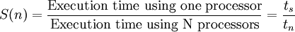
where  is the execution time on a single processor and
  is the execution time on a parallel computer.
S(n) therefore describes the scalability of the system as the number of processors is increased. The ideal speedup is n when using n processors, i.e. when the computations can be divided into equal duration processes with each process running on one processor (with no communication overhead). Ironically, this is called embarrassingly parallel computing!
In some cases, superlinear speedup (S(n)>n) may be encountered. Usually this is caused by either using a suboptimal sequential algorithm or some unique specification of the hardware architecture that favors the parallel computation. For example, one common reason for superlinear speedup is the extra memory in the multiprocessor system.
The speedup of any parallel computing environment obeys the Amdahl's Law.
Amdahl's law states that if F is the fraction of a calculation that is sequential (i.e. cannot benefit from parallelisation), and (1 − F) is the fraction that can be parallelised, then the maximum speedup that can be achieved by using N processors is
 .
.
In the limit, as N tends to infinity, the maximum speedup tends to 1/F. In practice, price/performance ratio falls rapidly as N is increased once (1 − F)/N is small compared to F.
As an example, if F is only 10%, the problem can be sped up by only a maximum of a factor of 10, no matter how large the value of N used. For this reason, parallel computing is only useful for either small numbers of processors, or problems with very low values of F: so-called embarrassingly parallel problems. A great part of the craft of parallel programming consists of attempting to reduce F to the smallest possible value.
Efficiency
The efficiency of a parallel system describes the fraction of the time that is being used by the processors for a given computation. It is defined as

which yields the following

For example, if E = 50%, the processors are being used half of the time to perform the actual computation.
Cost
The cost of a computation in a parallel environment is defined as the product of the number of processors used times the total execution time

The above equation can be written as a function of the efficiency by using the fact that  which yields
Performance of CFD codes
The method used to assess the performance of a parallel CFD solver is becoming a topic for debate. While some implementations use a fixed number of outer iterations to assess the performance of the parallel solver regardless of whether a solution has ben obtained or not, other implementors use a fixed value for the residual as a basis for evaluation. Ironically, a large amount of implementors do not mention the method used in their assessment!
The reason for this discrepancy is that the first group (who uses a fixed number of outer iterations) believes that the evaluation of the parallel performance should be done using exactely the same algorithm which justifies the use of a fixed number of outer iterations. This can be acceptable from an algorithmic point of view.
The other group (who uses a fixed value for the maximum residual) believes that the evaluation of the parallel performance should be done using the converged solution of the problem which justifies the use of the maximum residual as a criterion for performance measurement. This is acceptable from an engineering point of view and from the user point of view. In all cases, the parallel code will be used to seek a valid solution! Now if the number of outer iterations is the same as that of the sequential version, tant mieux!
The problem becomes more complicated when an algebraic multigrid solver is used. Depending on the method used in implementing the AMG solver, the maximum number of AMG levels in the parallel version will usually be less than that of the sequential version which raises the issue that one is not comparing the same algorithm. From an engineering point of view, the main concern is to obtain a valid solution for a given problem in a reasonable amount of time and thus, a user will not actually perform a sequential run and then a parallel run; rather, she will require the code to use as many AMG levels as possible.
Message passing
In a distributed memory environment, Message Passing is a protocol used to exchange messages or copy data from one memory location to another (where each memory belongs to a different computer). One of the most popular protocols is called the Message Passing Interface, MPI.
Peer to peer communication
Peer to Peer (P2P) communication, as the name designates, occurs when one processor communicates with another processor at one time. Only these two processors are involved in the communication. There are two fundamental operations that take place in a P2P communication:
- A send operation
- A corresponding receive operation
P2P communication can be performed using either a blocking or a non-blocking method.
Blocking
A blocking message occurs when one of the processors performs a send operation and does not return (i.e. does not execute any following instruction) unless it is sure that the message buffer can be reclaimed.

Non-blocking
A non-blocking message is the opposite of a blocking message where a processor performs a send or a receive operation and immediately returns (to the next instruction in the code) without caring whether the message has been received or not. Such a communication is shown in the figure below.

Advice
Both of the above communication methods have their own set of advantages and disadvantages.
For a blocking communication, one is almost certain that a given message will be received at its destination; however, the major problem with such a communication is that it requires the allocation of additional buffer memory which is not always available for large messages. On the other hand, an immediate communication does not have this problem (since the message waits till it has enough memory to be sent) but one is not always certain that the message will be received at its destination. Of course, designing a parallel program is not a game of luck. Both methods can be used successfully if they are carefully implemented in the code. For instance, in a parallel CFD code based on domain decomposition, there will be an inter-processor communication at some point. The best way to do this communication is to use a non-blocking method as the blocking method will end up with a dead lock (depending on the topology of the partitions).
So, as a general rule, when two processors know where to send and from who to receive, a blocking operation can be used. For example, when the master processor is distributing the initial data in the mesh, a blocking operation can be used here.
Collective communication
In collective communication, all the processors are involved with some kind of send and/or receive operations. However, this is not done by explicitly using send or receive operations since MPI provides an interface for collective communication. The mostly used collective communication routines are
- Broadcast
- Gather
- Reduce
Broadcast
A broadcast operation of consists of broadcasting or sending a message from a root processor to all other processors.

Gather
A gather operation of consists of gathering values from a group processors and doing something with them. For example, the Master processor might want to gather the solution from each processor to put them in one final array.
Reduce
In a reduce operation, the result is a reduction of values on all processors to a single value on a single processor using an algebraic/boolean operation such as a sum, a minimum, a maximum etc…

References
- Wilkinson, Barry and C. Michael Allen (1999), Parallel Programming : Techniques and Applications Using Networked Workstations and Parallel Computers, ISBN 0136717101, 1st Ed., Prentice Hall, Upper Saddle River, N.J..
Resources
- MPI Tutorial
- Course about MPI (in French)