Calculation on non-orthogonal curvelinear structured grids, finite-volume method
From CFD-Wiki
(Difference between revisions)
(→2D case) |
(→2D case) |
||
| Line 84: | Line 84: | ||
</math> | </math> | ||
</td><td width="5%">(12)</td></tr></table> | </td><td width="5%">(12)</td></tr></table> | ||
| + | |||
| + | <table width="70%"><tr><td> | ||
| + | :<math> | ||
| + | A^{\phi}_{N} = \left( \frac{ \Gamma }{J} \gamma \frac{\Delta \xi}{\Delta \eta} \right)_{n} + max \left[ 0, - \left( \rho V \Delta \xi \right)_{n} \right] | ||
| + | </math> | ||
| + | </td><td width="5%">(13)</td></tr></table> | ||
Revision as of 19:55, 19 August 2010
2D case
For calculations in complex geometries boundary-fitted non-orthogonal curvlinear grids is usually used.
General transport equation is transformed from the physical domain  into the computational domain
  as the following equation
|
| (2) |
![\frac{\partial}{\partial \xi} \left( \rho U \phi \right) + \frac{\partial }{ \partial \eta } \left( \rho V \phi \right) = \frac{\partial}{\partial \xi} \left[ \frac{\Gamma }{J} \left( \alpha \frac{\partial \phi}{\partial \xi} - \beta \frac{\partial \phi}{ \partial \eta} \right) \right] + \frac{\partial}{\partial \eta} \left[ \frac{\Gamma}{J} \left( \gamma \frac{\partial \phi}{\partial \eta} - \beta \frac{\partial \phi}{ \partial \xi} \right) \right] + J S^{\phi}](/W/images/math/3/8/2/382456ea15e881910f1b040f17a347bd.png)
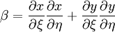
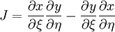
where
|
| (3) |
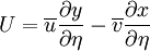
|
| (4) |
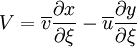
|
| (5) |
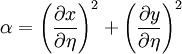
|
| (6) |
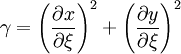
|
| (7) |
|
| (8) |
Using the finite volume method the trnsformed equations can be integrated as follows:
|
| (9) |
![\left[ \left( \rho U \Delta \eta \right) \right]^{e}_{w} + \left[ \left( \rho V \Delta \xi \right) \right]^{n}_{s} = \left[ \frac{\Gamma \Delta \eta}{J} \left( \alpha \frac{\partial \phi}{\partial \xi} - \beta \frac{\partial \phi}{ \partial \eta} \right) \right]^{e}_{w} + \left[ \frac{\Gamma \Delta \xi}{J} \left( \gamma \frac{\partial \phi}{\partial \eta } - \beta \frac{\partial \phi}{\partial \xi} \right) \right]^{n}_{s} + \left( J \Delta \xi \Delta \eta \right) \overline{S}^{\phi}_{P}](/W/images/math/c/9/b/c9bc323ba9595d8d85677016f4e53536.png)
The convection terms are approximated as described in section http://www.cfd-online.com/Wiki/Discretization_of_the_convection_term .
Diffusion terms are approximated by the second-oder central differencing scheme.
The standard form of the finite volume equation can be obtained as
|
| (10) |

where
|
| (11) |
![A^{\phi}_{E} = \left(\frac{\Gamma}{J} \alpha \frac{\Delta \eta}{\Delta \xi} \right)_{e} + max \left[ 0, - \left( \rho U \Delta \eta \right)_{e} \right]](/W/images/math/d/d/3/dd391b55e6d5ab853dfb8a363e1ad14e.png)
|
| (12) |
![A^{\phi}_{W} = \left(\frac{\Gamma}{J} \alpha \frac{\Delta \eta}{\Delta \xi} \right)_{w} + max \left[ 0, \left( \rho U \Delta \eta \right)_{w} \right]](/W/images/math/0/d/b/0dbf08dd7c67f1ce5b898703ed51ba9e.png)
|
| (13) |
![A^{\phi}_{N} = \left( \frac{ \Gamma }{J} \gamma \frac{\Delta \xi}{\Delta \eta} \right)_{n} + max \left[ 0, - \left( \rho V \Delta \xi \right)_{n} \right]](/W/images/math/7/c/1/7c191e197bd433da99e710d3972cb506.png)