|
|
| (27 intermediate revisions not shown) |
| Line 1: |
Line 1: |
| - | Lid-driven cavity using pressure-free velocity formulation | + | ==Lid-driven cavity using pressure-free velocity formulation== |
| | | | |
| - | <pre>
| + | This sample code uses four-node simple-cubic finite elements and simple iteration. |
| - | %LDCW LID-DRIVEN CAVITY
| + | |
| - | % Finite element solution of the 2D Navier-Stokes equation using 4-node, 12 DOF,
| + | |
| - | % (3-DOF/node), simple-cubic-derived rectangular Hermite basis for
| + | |
| - | % the Lid-Driven Cavity problem.
| + | |
| - | %
| + | |
| - | % This could also be characterized as a VELOCITY-STREAM FUNCTION or
| + | |
| - | % STREAM FUNCTION-VELOCITY method.
| + | |
| - | %
| + | |
| - | % Reference: "A Hermite finite element method for incompressible fluid flow",
| + | |
| - | % Int. J. Numer. Meth. Fluids, 64, P376-408 (2010).
| + | |
| - | %
| + | |
| - | % Simplified Wiki version
| + | |
| - | % The rectangular problem domain is defined between Cartesian
| + | |
| - | % coordinates Xmin & Xmax and Ymin & Ymax.
| + | |
| - | % The computational grid has NumEx elements in the x-direction
| + | |
| - | % and NumEy elements in the y-direction.
| + | |
| - | % The nodes and elements are numbered column-wise from the
| + | |
| - | % upper left corner to the lower right corner.
| + | |
| - | %
| + | |
| - | %This script calls the user-defined functions:
| + | |
| - | % regrade - to regrade the mesh
| + | |
| - | % DMatW - to evaluate element diffusion matrix
| + | |
| - | % CMatW - to evaluate element convection matrix
| + | |
| - | % GetPresW - to evaluate the pressure
| + | |
| - | % ilu_gmres_with_EBC - to solve the system with essential/Dirichlet BCs
| + | |
| - | %
| + | |
| - | % Jonas Holdeman August 2007, revised June 2011
| + | |
| | | | |
| - | clear all;
| + | ===Theory=== |
| - | disp('Lid-driven cavity');
| + | The incompressible Navier-Stokes equation is a differential algebraic equation, having the inconvenient feature that there is no explicit mechanism for advancing the pressure in time. Consequently, much effort has been expended to eliminate the pressure from all or part of the computational process. We show a simple, natural way of doing this. |
| - | disp(' Four-node, 12 DOF, simple-cubic stream function basis.');
| + | |
| | | | |
| - | % -------------------------------------------------------------
| + | The incompressible Navier-Stokes equation is composite, the sum of two orthogonal equations, |
| - | nd = 3; nd2=nd*nd; % Number of DOF per node - do not change!!
| + | :<math>\frac{\partial\mathbf{v}}{\partial t}=\Pi^S(-\mathbf{v}\cdot\nabla\mathbf{v}+\nu\nabla^2\mathbf{v})+\mathbf{f}^S </math>, |
| - | % -------------------------------------------------------------
| + | :<math>\rho^{-1}\nabla p=\Pi^I(-\mathbf{v}\cdot\nabla\mathbf{v}+\nu\nabla^2\mathbf{v})+\mathbf{f}^I </math>, |
| - | ETstart=clock;
| + | where <math>\Pi^S</math> and <math>\Pi^I</math> are solenoidal and irrotational projection operators satisfying <math>\Pi^S+\Pi^I=1</math> and |
| | + | <math>\mathbf{f}^S</math> and <math>\mathbf{f}^I</math> are the nonconservative and conservative parts of the body force. This result follows from the Helmholtz Theorem . The first equation is a pressureless governing equation for the velocity, while the second equation for the pressure is a functional of the velocity and is related to the pressure Poisson equation. The explicit functional forms of the projection operator in 2D and 3D are found from the Helmholtz Theorem, showing that these are integro-differential equations, and not particularly convenient for numerical computation. |
| | | | |
| - | % Parameters for GMRES solver
| + | Equivalent weak or variational forms of the equations, proved to produce the same velocity solution as the Navier-Stokes equation are |
| - | GMRES.Tolerance=1.e-14;
| + | :<math>(\mathbf{w},\frac{\partial\mathbf{v}}{\partial t})=-(\mathbf{w},\mathbf{v}\cdot\nabla\mathbf{v})-\nu(\nabla\mathbf{w}: \nabla\mathbf{v})+(\mathbf{w},\mathbf{f}^S)</math>, |
| - | GMRES.MaxIterates=20;
| + | :<math>(\mathbf{g}_i,\nabla p)=-(\mathbf{g}_i,\mathbf{v}\cdot\nabla\mathbf{v}_j)-\nu(\nabla\mathbf{g}_i: \nabla\mathbf{v}_j)+(\mathbf{g}_i,\mathbf{f}^I)\,</math>, |
| - | GMRES.MaxRestarts=6;
| + | |
| | | | |
| - | % Optimal relaxation parameters for given Reynolds number
| + | for divergence-free test functions <math>\mathbf{w}</math> and irrotational test functions <math>\mathbf{g}</math> satisfying appropriate boundary conditions. Here, the projections are accomplished by the orthogonality of the solenoidal and irrotational function spaces. The discrete form of this is emminently suited to finite element computation of divergence-free flow. |
| - | % (see IJNMF reference)
| + | |
| - | % Re 100 1000 3200 5000 7500 10000 12500
| + | |
| - | % RelxFac: 1.04 1.11 .860 .830 .780 .778 .730
| + | |
| - | % ExpCR1 1.488 .524 .192 .0378 -- -- --
| + | |
| - | % ExpCRO 1.624 .596 .390 .331 .243 .163 .133
| + | |
| - | % CritFac: 1.82 1.49 1.14 1.027 .942 .877 .804
| + | |
| | | | |
| - | % Define the problem geometry, set mesh bounds:
| + | In the discrete case, it is desirable to choose basis functions for the velocity which reflect the essential feature of incompressible flow — the velocity elements must be divergence-free. While the velocity is the variable of interest, the existence of the stream function or vector potential is necessary by the Helmholtz Theorem. Further, to determine fluid flow in the absence of a pressure gradient, one can specify the difference of stream function values across a 2D channel, or the line integral of the tangential component of the vector potential around the channel in 3D, the flow being given by Stokes' Theorem. This leads naturally to the use of Hermite stream function (in 2D) or velocity potential elements (in 3D). |
| - | Xmin = 0.0; Xmax = 1.0; Ymin = 0.0; Ymax = 1.0;
| + | |
| | | | |
| - | % Set mesh grading parameters (set to 1 if no grading).
| + | Involving, as it does, both stream function and velocity degrees-of-freedom, the method might be called a '''velocity-stream function''' or '''stream function-velocity''' method. |
| - | % See below for explanation of use of parameters.
| + | |
| - | xgrd = .75; ygrd=.75; % (xgrd = 1, ygrd=1 for uniform mesh)
| + | |
| | | | |
| - | % Set " RefineBoundary=1 " for additional refinement at boundary,
| + | We now restrict discussion to 2D continuous Hermite finite elements which have at least first-derivative degrees-of-freedom. With this, one can draw a large number of candidate triangular and rectangular elements from the plate-bending literature. These elements have derivatives as components of the gradient. In 2D, the gradient and curl of a scalar are clearly orthogonal, given by the expressions, |
| - | % i.e., split first element along boundary into two.
| + | :<math>\nabla\phi = \left[\frac{\partial \phi}{\partial x},\,\frac{\partial \phi}{\partial y}\right]^T, \quad |
| - | RefineBoundary=1;
| + | \nabla\times\phi = \left[\frac{\partial \phi}{\partial y},\,-\frac{\partial \phi}{\partial x}\right]^T. </math> |
| | | | |
| - | % DEFINE THE MESH
| + | Adopting continuous plate-bending elements, interchanging the derivative degrees-of-freedom and changing the sign of the |
| - | % Set number of elements in each direction
| + | appropriate one gives many families of stream function elements. |
| - | NumEx = 16; NumEy = NumEx;
| + | |
| | | | |
| - | % PLEASE CHANGE OR SET NUMBER OF ELEMENTS TO CHANGE/SET NUMBER OF NODES!
| + | Taking the curl of the scalar stream function elements gives divergence-free velocity elements [1][2][5]. The requirement that the stream function elements be continuous assures that the normal component of the velocity is continuous across element interfaces, all that is necessary for vanishing divergence on these interfaces. |
| - | NumNx=NumEx+1; NumNy=NumEy+1;
| + | |
| | | | |
| - | % Define problem parameters:
| + | Boundary conditions are simple to apply. The stream function is constant on no-flow surfaces, with no-slip velocity conditions on surfaces. Stream function differences across open channels determine the flow. No boundary conditions are necessary on open boundaries [1], though consistent values may be used with some problems. These are all Dirichlet conditions. |
| - | % Lid velocity
| + | |
| - | Vlid=1.;
| + | |
| | | | |
| - | % Reynolds number
| + | The algebraic equations to be solved are simple to set up, but of course are non-linear, requiring iteration of the linearized equations. |
| - | Re=1000.;
| + | |
| | | | |
| - | % factor for under/over-relaxation starting at iteration RelxStrt
| + | The finite elements we will use here are apparently due to Melosh [3], but can also be found in Zienkiewitz [4]. These simple cubic-complete elements have three degrees-of-freedom at each of the four nodes. In the sample code we use this Hermite element for the pressure, and the modified form obtained by interchanging derivatives and the sign of one of them (though a simple bilinear element could be used for the pressure as well). The degrees-of-freedom are the pressure and pressure gardient, and the stream function and components of the solenoidal velocity for the modified element. The normal component of the velocity is continuous at element interfaces as is required, but the tangential velocity component may not be continuous. |
| - | RelxFac = 1.; %
| + | |
| | | | |
| - | % Number of nonlinear iterations
| + | The code implementing the lid-driven cavity problem is written for Matlab. The script below is problem-specific, and calls problem-independent functions to evaluate the element diffusion and convection matricies and evaluate the pressure from the resulting velocity field. These three functions accept general quadrilateral elements with straight sides as well as the rectangular elements used here. Other functions are a GMRES iterative solver using ILU preconditioning and incorporating the essential boundary conditions, and a function to produce non-uniform nodal spacing for the problem mesh. |
| - | MaxNLit=10; %
| + | |
| | | | |
| - | %--------------------------------------------------------
| + | This "educational code" is a simplified version of the code used in [1]. The user interface is the code itself. The user can experiment with changing the mesh, the Reynolds number, and the number of nonlinear iterations performed, as well as the relaxation factor. There are suggestions in the code regarding near-optimum choices for this factor as a function of Reynolds number. These values are given in the paper as well. For larger Reynolds numbers, a smaller relaxation factor speeds up convergence by smoothing the velocity factor <math>(\mathbf{v}\cdot\nabla)</math> in the convection term, but will impede convergence if made too small. |
| | | | |
| - | % Viscosity for specified Reynolds number
| + | The output consists of graphic plots of contour levels of the stream function and the pressure levels. |
| - | nu=Vlid*(Xmax-Xmin)/Re;
| + | |
| - |
| + | |
| - | % Grade the mesh spacing if desired, call regrade(x,agrd,e).
| + | |
| - | % if e=0: refine both sides, 1: refine upper, 2: refine lower
| + | |
| - | % if agrd=xgrd|ygrd is the parameter which controls grading, then
| + | |
| - | % if agrd=1 then leave array unaltered.
| + | |
| - | % if agrd<1 then refine (make finer) towards the ends
| + | |
| - | % if agrd>1 then refine (make finer) towards the center.
| + | |
| - | %
| + | |
| - | % Generate equally-spaced nodal coordinates and refine if desired.
| + | |
| - | if (RefineBoundary==1)
| + | |
| - | XNc=linspace(Xmin,Xmax,NumNx-2);
| + | |
| - | XNc=[XNc(1),(.62*XNc(1)+.38*XNc(2)),XNc(2:end-1),(.38*XNc(end-1)+.62*XNc(end)),XNc(end)];
| + | |
| - | YNc=linspace(Ymax,Ymin,NumNy-2);
| + | |
| - | YNc=[YNc(1),(.62*YNc(1)+.38*YNc(2)),YNc(2:end-1),(.38*YNc(end-1)+.62*YNc(end)),YNc(end)];
| + | |
| - | else
| + | |
| - | XNc=linspace(Xmin,Xmax,NumNx);
| + | |
| - | YNc=linspace(Ymax,Ymin,NumNy);
| + | |
| - | end
| + | |
| - | if xgrd ~= 1 XNc=regrade(XNc,xgrd,0); end; % Refine mesh if desired
| + | |
| - | if ygrd ~= 1 YNc=regrade(YNc,ygrd,0); end;
| + | |
| - | [Xgrid,Ygrid]=meshgrid(XNc,YNc);% Generate the x- and y-coordinate meshes.
| + | |
| | | | |
| - | % Allocate storage for fields
| + | A simplified version for this Wiki resulted from removal of computation of the vorticity, a restart capability, area weighting for the error, and production of publication-quality plots from one of the research codes used with the paper. |
| - | psi0=zeros(NumNy,NumNx);
| + | |
| - | u0=zeros(NumNy,NumNx);
| + | |
| - | v0=zeros(NumNy,NumNx);
| + | |
| | | | |
| - | %--------------------Begin grid plot-----------------------
| + | This modified version posted 3/15/2013 updates the code to MatLab version R2012b. The element properties are now defined in classes, and the code has been modified to accept class definitions for additional quartic and quintic divergence-free elements on quadrilaterals and quadratic and quartic divergence-free elements on triangles. |
| - | % ********************** FIGURE 1 *************************
| + | |
| - | % Plot the grid
| + | |
| - | figure(1);
| + | |
| - | clf;
| + | |
| - | orient portrait; orient tall;
| + | |
| - | subplot(2,2,1);
| + | |
| - | hold on;
| + | |
| - | plot([Xmax;Xmin],[YNc;YNc],'k');
| + | |
| - | plot([XNc;XNc],[Ymax;Ymin],'k');
| + | |
| - | hold off;
| + | |
| - | axis([Xmin,Xmax,Ymin,Ymax]);
| + | |
| - | axis equal;
| + | |
| - | axis image;
| + | |
| - | title([num2str(NumNx) 'x' num2str(NumNy) ...
| + | |
| - | ' node mesh for Lid-driven cavity']);
| + | |
| - | pause(.1);
| + | |
| - | %-------------- End plotting Figure 1 ----------------------
| + | |
| | | | |
| - | | + | ===Lid-driven cavity Matlab script=== |
| - | %Contour levels, Ghia, Ghia & Shin, Re=100, 400, 1000, 3200, ...
| + | |
| - | clGGS=[-.1175,-.1150,-.11,-.1,-.09,-.07,-.05,-.03,-.01,-1.e-4,-1.e-5,-1.e-7,-1.e-10,...
| + | |
| - | 1.e-8,1.e-7,1.e-6,1.e-5,5.e-5,1.e-4,2.5e-4,5.e-4,1.e-3,1.5e-3,3.e-3];
| + | |
| - | CL=clGGS; % Select contour level option
| + | |
| - | if (Vlid<0) CL=-CL; end
| + | |
| - | | + | |
| - | NumNod=NumNx*NumNy; % total number of nodes
| + | |
| - | MaxDof=nd*NumNod; % maximum number of degrees of freedom
| + | |
| - | EBC.Mxdof=nd*NumNod; % maximum number of degrees of freedom
| + | |
| - | | + | |
| - | nn2nft=zeros(2,NumNod); % node number -> nf & nt
| + | |
| - | NodNdx=zeros(2,NumNod);
| + | |
| - | % Generate lists of active nodal indices, freedom number & type
| + | |
| - | ni=0; nf=-nd+1; nt=1; % ________
| + | |
| - | for nx=1:NumNx % | |
| + | |
| - | for ny=1:NumNy % | |
| + | |
| - | ni=ni+1; % |________|
| + | |
| - | NodNdx(:,ni)=[nx;ny];
| + | |
| - | nf=nf+nd; % all nodes have 4 dofs
| + | |
| - | nn2nft(:,ni)=[nf;nt]; % dof number & type (all nodes type 1)
| + | |
| - | end;
| + | |
| - | end;
| + | |
| - | %NumNod=ni; % total number of nodes
| + | |
| - | nf2nnt=zeros(2,MaxDof); % (node, type) associated with dof
| + | |
| - | ndof=0; dd=[1:nd];
| + | |
| - | for n=1:NumNod
| + | |
| - | for k=1:nd
| + | |
| - | nf2nnt(:,ndof+k)=[n;k];
| + | |
| - | end
| + | |
| - | ndof=ndof+nd;
| + | |
| - | end
| + | |
| - | | + | |
| - | NumEl=NumEx*NumEy;
| + | |
| - | | + | |
| - | % Generate element connectivity, from upper left to lower right.
| + | |
| - | Elcon=zeros(4,NumEl);
| + | |
| - | ne=0; LY=NumNy;
| + | |
| - | for nx=1:NumEx
| + | |
| - | for ny=1:NumEy
| + | |
| - | ne=ne+1;
| + | |
| - | Elcon(1,ne)=1+ny+(nx-1)*LY;
| + | |
| - | Elcon(2,ne)=1+ny+nx*LY;
| + | |
| - | Elcon(3,ne)=1+(ny-1)+nx*LY;
| + | |
| - | Elcon(4,ne)=1+(ny-1)+(nx-1)*LY;
| + | |
| - | end % loop on ny
| + | |
| - | end % loop on nx
| + | |
| - | | + | |
| - | % Begin essential boundary conditions, allocate space
| + | |
| - | MaxEBC = nd*2*(NumNx+NumNy-2);
| + | |
| - | EBC.dof=zeros(MaxEBC,1); % Degree-of-freedom index
| + | |
| - | EBC.typ=zeros(MaxEBC,1); % Dof type (1,2,3)
| + | |
| - | EBC.val=zeros(MaxEBC,1); % Dof value
| + | |
| - | | + | |
| - | X1=XNc(2); X2=XNc(NumNx-1);
| + | |
| - | nc=0;
| + | |
| - | for nf=1:MaxDof
| + | |
| - | ni=nf2nnt(1,nf);
| + | |
| - | nx=NodNdx(1,ni);
| + | |
| - | ny=NodNdx(2,ni);
| + | |
| - | x=XNc(nx);
| + | |
| - | y=YNc(ny);
| + | |
| - | if(x==Xmin | x==Xmax | y==Ymin)
| + | |
| - | nt=nf2nnt(2,nf);
| + | |
| - | switch nt;
| + | |
| - | case {1, 2, 3}
| + | |
| - | nc=nc+1; EBC.typ(nc)=nt; EBC.dof(nc)=nf; EBC.val(nc)=0; % psi, u, v
| + | |
| - | end % switch (type)
| + | |
| - | elseif (y==Ymax)
| + | |
| - | nt=nf2nnt(2,nf);
| + | |
| - | switch nt;
| + | |
| - | case {1, 3}
| + | |
| - | nc=nc+1; EBC.typ(nc)=nt; EBC.dof(nc)=nf; EBC.val(nc)=0; % psi, v
| + | |
| - | case 2
| + | |
| - | nc=nc+1; EBC.typ(nc)=nt; EBC.dof(nc)=nf; EBC.val(nc)=Vlid; % u
| + | |
| - | end % switch (type)
| + | |
| - | end % if (boundary)
| + | |
| - | end % for nf
| + | |
| - | EBC.num=nc;
| + | |
| - |
| + | |
| - | if (size(EBC.typ,1)>nc) % Truncate arrays if necessary
| + | |
| - | EBC.typ=EBC.typ(1:nc);
| + | |
| - | EBC.dof=EBC.dof(1:nc);
| + | |
| - | EBC.val=EBC.val(1:nc);
| + | |
| - | end % End ESSENTIAL (Dirichlet) boundary conditions
| + | |
| - | | + | |
| - | % partion out essential (Dirichlet) dofs
| + | |
| - | p_vec = [1:EBC.Mxdof]'; % List of all dofs
| + | |
| - | EBC.p_vec_undo = zeros(1,EBC.Mxdof);
| + | |
| - | % form a list of non-diri dofs
| + | |
| - | EBC.ndro = p_vec(~ismember(p_vec, EBC.dof)); % list of non-diri dofs
| + | |
| - | % calculate p_vec_undo to restore Q to the original dof ordering
| + | |
| - | EBC.p_vec_undo([EBC.ndro;EBC.dof]) = [1:EBC.Mxdof]; %p_vec';
| + | |
| - | | + | |
| - | Q=zeros(MaxDof,1); % Allocate space for solution (dof) vector
| + | |
| - | | + | |
| - | % Initialize fields to boundary conditions
| + | |
| - | for k=1:EBC.num
| + | |
| - | Q(EBC.dof(k))=EBC.val(k);
| + | |
| - | end;
| + | |
| - | | + | |
| - | errpsi=zeros(NumNy,NumNx); % error correct for iteration
| + | |
| - | | + | |
| - | MxNL=max(1,MaxNLit);
| + | |
| - | np0=zeros(1,MxNL); % Arrays for convergence info
| + | |
| - | nv0=zeros(1,MxNL);
| + | |
| - | | + | |
| - | Qs=[];
| + | |
| - |
| + | |
| - | Dmat = spalloc(MaxDof,MaxDof,36*MaxDof); % to save the diffusion matrix
| + | |
| - | Vdof=zeros(nd,4);
| + | |
| - | Xe=zeros(2,4); % coordinates of element corners
| + | |
| - | | + | |
| - | NLitr=0; ND=1:nd;
| + | |
| - | while (NLitr<MaxNLit), NLitr=NLitr+1; % <<< BEGIN NONLINEAR ITERATION
| + | |
| - |
| + | |
| - | tclock=clock; % Start assembly time <<<<<<<<<
| + | |
| - | % Generate and assemble element matrices
| + | |
| - | Mat=spalloc(MaxDof,MaxDof,36*MaxDof);
| + | |
| - | RHS=spalloc(MaxDof,1,MaxDof);
| + | |
| - | %RHS = zeros(MaxDof,1);
| + | |
| - | Emat=zeros(1,16*nd2); % Values 144=4*4*(nd*nd)
| + | |
| - | | + | |
| - | % BEGIN GLOBAL MATRIX ASSEMBLY
| + | |
| - | for ne=1:NumEl
| + | |
| - |
| + | |
| - | for k=1:4
| + | |
| - | ki=NodNdx(:,Elcon(k,ne));
| + | |
| - | Xe(:,k)=[XNc(ki(1));YNc(ki(2))];
| + | |
| - | end
| + | |
| - |
| + | |
| - | if NLitr == 1
| + | |
| - | % Fluid element diffusion matrix, save on first iteration
| + | |
| - | [DEmat,Rndx,Cndx] = DMatW(Xe,Elcon(:,ne),nn2nft);
| + | |
| - | Dmat=Dmat+sparse(Rndx,Cndx,DEmat,MaxDof,MaxDof); % Global diffusion mat
| + | |
| - | end
| + | |
| - |
| + | |
| - | if (NLitr>1)
| + | |
| - | % Get stream function and velocities
| + | |
| - | for n=1:4
| + | |
| - | Vdof(ND,n)=Q((nn2nft(1,Elcon(n,ne))-1)+ND); % Loop over local element nodes
| + | |
| - | end
| + | |
| - | % Fluid element convection matrix, first iteration uses Stokes equation.
| + | |
| - | [Emat,Rndx,Cndx] = CMatW(Xe,Elcon(:,ne),nn2nft,Vdof);
| + | |
| - | Mat=Mat+sparse(Rndx,Cndx,-Emat,MaxDof,MaxDof); % Global convection assembly
| + | |
| - | end
| + | |
| - | | + | |
| - | end; % loop ne over elements
| + | |
| - | % END GLOBAL MATRIX ASSEMBLY
| + | |
| - | | + | |
| - | Mat = Mat -nu*Dmat; % Add in cached/saved global diffusion matrix
| + | |
| - | | + | |
| - | disp(['(' num2str(NLitr) ') Matrix assembly complete, elapsed time = '...
| + | |
| - | num2str(etime(clock,tclock)) ' sec']); % Assembly time <<<<<<<<<<<
| + | |
| - | pause(1);
| + | |
| - | | + | |
| - | Q0 = Q; % Save dof values
| + | |
| - | | + | |
| - | % Solve system
| + | |
| - | tclock=clock; %disp('start solution'); % Start solution time <<<<<<<<<<<<<<
| + | |
| - | | + | |
| - | RHSr=RHS(EBC.ndro)-Mat(EBC.ndro,EBC.dof)*EBC.val;
| + | |
| - | Matr=Mat(EBC.ndro,EBC.ndro);
| + | |
| - | Qs=Q(EBC.ndro);
| + | |
| - | | + | |
| - | Qr=ilu_gmres_with_EBC(Matr,RHSr,[],GMRES,Qs);
| + | |
| - | | + | |
| - | Q=[Qr;EBC.val]; % Augment active dofs with esential (Dirichlet) dofs
| + | |
| - | Q=Q(EBC.p_vec_undo); % Restore natural order
| + | |
| - |
| + | |
| - | stime=etime(clock,tclock); % Solution time <<<<<<<<<<<<<<
| + | |
| - | | + | |
| - | % ****** APPLY RELAXATION FACTOR *********************
| + | |
| - | if(NLitr>1) Q=RelxFac*Q+(1-RelxFac)*Q0; end
| + | |
| - | % ****************************************************
| + | |
| - | | + | |
| - | % Compute change and copy dofs to field arrays
| + | |
| - | dsqp=0; dsqv=0;
| + | |
| - | for k=1:MaxDof
| + | |
| - | ni=nf2nnt(1,k); nx=NodNdx(1,ni); ny=NodNdx(2,ni);
| + | |
| - | switch nf2nnt(2,k) % switch on dof type
| + | |
| - | case 1
| + | |
| - | dsqp=dsqp+(Q(k)-Q0(k))^2; psi0(ny,nx)=Q(k);
| + | |
| - | errpsi(ny,nx)=Q0(k)-Q(k);
| + | |
| - | case 2
| + | |
| - | dsqv=dsqv+(Q(k)-Q0(k))^2; u0(ny,nx)=Q(k);
| + | |
| - | case 3
| + | |
| - | dsqv=dsqv+(Q(k)-Q0(k))^2; v0(ny,nx)=Q(k);
| + | |
| - | end % switch on dof type
| + | |
| - | end % for
| + | |
| - | np0(NLitr)=sqrt(dsqp);
| + | |
| - | nv0(NLitr)=sqrt(dsqv);
| + | |
| - | | + | |
| - | if (np0(NLitr)<=1e-15|nv0(NLitr)<=1e-15)
| + | |
| - | MaxNLit=NLitr; np0=np0(1:MaxNLit); nv0=nv0(1:MaxNLit); end;
| + | |
| - | disp(['(' num2str(NLitr) ') Solution time for linear system = '...
| + | |
| - | num2str(etime(clock,tclock)) ' sec']); % Solution time <<<<<<<<<<<<
| + | |
| - |
| + | |
| - | %---------- Begin plot of intermediate results ----------
| + | |
| - | % ********************** FIGURE 2 *************************
| + | |
| - | figure(1);
| + | |
| - | | + | |
| - | % Stream function (intermediate)
| + | |
| - | subplot(2,2,3);
| + | |
| - | contour(Xgrid,Ygrid,psi0,8,'k'); % Plot contours (trajectories)
| + | |
| - | axis([Xmin,Xmax,Ymin,Ymax]);
| + | |
| - | title(['Lid-driven cavity, Re=' num2str(Re)]);
| + | |
| - | axis equal; axis image;
| + | |
| - | | + | |
| - | % Plot convergence info
| + | |
| - | subplot(2,2,2);
| + | |
| - | semilogy(1:NLitr,nv0(1:NLitr),'k-+',1:NLitr,np0(1:NLitr),'k-o');
| + | |
| - | xlabel('Nonlinear iteration number');
| + | |
| - | ylabel('Nonlinear correction');
| + | |
| - | axis square;
| + | |
| - | title(['Iteration conv., Re=' num2str(Re)]);
| + | |
| - | legend('U','Psi');
| + | |
| - | | + | |
| - | % Plot nonlinear iteration correction contours
| + | |
| - | subplot(2,2,4);
| + | |
| - | contour(Xgrid,Ygrid,errpsi,8,'k'); % Plot contours (trajectories)
| + | |
| - | axis([Xmin,Xmax,Ymin,Ymax]);
| + | |
| - | axis equal; axis image;
| + | |
| - | title(['Iteration correction']);
| + | |
| - | pause(1);
| + | |
| - | % ********************** END FIGURE 2 *************************
| + | |
| - | %---------- End plot of intermediate results ---------
| + | |
| - | | + | |
| - | if (nv0(NLitr)<1e-15) break; end % Terminate iteration if non-significant
| + | |
| - | | + | |
| - | end; % <<< (while) END NONLINEAR ITERATION
| + | |
| - | | + | |
| - | format short g;
| + | |
| - | disp('Convergence results by iteration: velocity, stream function');
| + | |
| - | disp(['nv0: ' num2str(nv0)]); disp(['np0: ' num2str(np0)]);
| + | |
| - | | + | |
| - | % >>>>>>>>>>>>>> BEGIN PRESSURE RECOVERY <<<<<<<<<<<<<<<<<<
| + | |
| - | % Essential pressure boundary condition
| + | |
| - | % Index of node to apply pressure BC, value at node
| + | |
| - | PBCnx=fix((NumNx+1)/2); % Apply at center of mesh
| + | |
| - | PBCny=fix((NumNy+1)/2);
| + | |
| - | PBCnod=0;
| + | |
| - | for k=1:NumNod
| + | |
| - | if (NodNdx(1,k)==PBCnx & NodNdx(2,k)==PBCny) PBCnod=k; break; end
| + | |
| - | end
| + | |
| - | if (PBCnod==0) error('Pressure BC node not found');
| + | |
| - | else
| + | |
| - | EBCp.nodn = [PBCnod]; % Pressure BC node number
| + | |
| - | EBCp.val = [0]; % set P = 0.
| + | |
| - | end
| + | |
| - | % Cubic pressure
| + | |
| - | [P,Px,Py] = GetPresW(NumNod,NodNdx,Elcon,nn2nft,Xgrid,Ygrid,Q,EBCp,nu);
| + | |
| - | % ******************** END PRESSURE RECOVERY *********************
| + | |
| - | | + | |
| - | % ********************** CONTINUE FIGURE 1 *************************
| + | |
| - | figure(1);
| + | |
| - | | + | |
| - | % Stream function (final)
| + | |
| - | subplot(2,2,3);
| + | |
| - | [CT,hn]=contour(Xgrid,Ygrid,psi0,CL,'k'); % Plot contours (trajectories)
| + | |
| - | clabel(CT,hn,CL([1,3,5,7,9,10,11,19,23]));
| + | |
| - | hold on;
| + | |
| - | plot([Xmin,Xmin,Xmax,Xmax,Xmin],[Ymax,Ymin,Ymin,Ymax,Ymax],'k');
| + | |
| - | hold off;
| + | |
| - | axis([Xmin,Xmax,Ymin,Ymax]);
| + | |
| - | axis equal; axis image;
| + | |
| - | title(['Stream lines, ' num2str(NumNx) 'x' num2str(NumNy) ...
| + | |
| - | ' mesh, Re=' num2str(Re)]);
| + | |
| - | | + | |
| - | % Plot pressure contours (final)
| + | |
| - | subplot(2,2,4);
| + | |
| - | CPL=[-.002,0,.02,.05,.07,.09,.11,.12,.17,.3];
| + | |
| - | [CT,hn]=contour(Xgrid,Ygrid,P,CPL,'k'); % Plot pressure contours
| + | |
| - | clabel(CT,hn,CPL([3,5,7,10]));
| + | |
| - | hold on;
| + | |
| - | plot([Xmin,Xmin,Xmax,Xmax,Xmin],[Ymax,Ymin,Ymin,Ymax,Ymax],'k');
| + | |
| - | hold off;
| + | |
| - | axis([Xmin,Xmax,Ymin,Ymax]);
| + | |
| - | axis equal; axis image;
| + | |
| - | title(['Simple cubic pressure contours, Re=' num2str(Re)]);
| + | |
| - | % ********************* END FIGURE 1 *************************
| + | |
| - | | + | |
| - | disp(['Total elapsed time = '...
| + | |
| - | num2str(etime(clock,ETstart)/60) ' min']); % Elapsed time from start <<<
| + | |
| - | </pre>
| + | |
| | <pre> | | <pre> |
| - | function [Dm,RowNdx,ColNdx]=DMatW(Xe,Elcon,nn2nft)
| + | %LDC3W LID-DRIVEN CAVITY |
| - | %DMATW - Returns the affine-mapped element diffusion matrix for the simple cubic Hermite | + | % Finite element solution of the 2D Navier-Stokes equation using 4-node, |
| - | % basis functions on 4-node straight-sided quadrilateral elements with 3 DOF | + | % 12 DOF, (3-DOF/node), simple-cubic-derived rectangular Hermite basis for |
| - | % per node using Gauss quadrature on the reference square and row/col indices. | + | % the Lid-Driven Cavity problem. |
| - | | + | |
| | % | | % |
| - | % Cubic-complete, fully-conforming, divergence-free, Hermite basis | + | % This could also be characterized as a VELOCITY-STREAM FUNCTION or |
| - | % functions on 4-node rectangular elements with 3 DOF per node using | + | % STREAM FUNCTION-VELOCITY method. |
| - | % Gauss quadrature on the 2x2 reference square.
| + | |
| - | % The assumed nodal numbering starts with 1 at the lower left corner
| + | |
| - | % of the element and proceeds counter-clockwise around the element.
| + | |
| - | % Uses second derivatives of stream function.
| + | |
| | % | | % |
| - | % Usage: | + | % Reference: "A Hermite finite element method for incompressible fluid flow", |
| - | % [Dm,Rndx,Cndx] = DMatW(Xe,Elcon,nn2nft)
| + | % Int. J. Numer. Meth. Fluids, 64, P376-408 (2010). |
| - | % Xe(1,:) - x-coordinates of corner nodes of element.
| + | |
| - | % Xe(2,:) - y-coordinates of corner nodes of element.
| + | |
| - | % and shape of the element. It is constant for affine elements. | + | |
| - | % Elcon - connectivity matrix for this element.
| + | |
| - | % nn2nft - global number and type of DOF at each node
| + | |
| | % | | % |
| - | % Jonas Holdeman, August 2007, revised June 2011 | + | % Simplified Wiki version |
| - | | + | % The rectangular problem domain is defined between Cartesian |
| - | % Constants and fixed data | + | % coordinates Xmin & Xmax and Ymin & Ymax. |
| - | nd = 3; nd4=4*nd; ND=1:nd; % nd = number of dofs per node,
| + | % The computational grid has NumEx elements in the x-direction |
| - | nn=[-1 -1; 1 -1; 1 1; -1 1]; % defines local nodal order
| + | % and NumEy elements in the y-direction. |
| - | | + | % The nodes and elements are numbered column-wise from the |
| - | % Define 4-point quadrature data once, on first call.
| + | % upper left corner to the lower right corner. |
| - | % Gaussian weights and absissas to integrate 7th degree polynomials exactly.
| + | |
| - | global GQ4;
| + | |
| - | if (isempty(GQ4)) % Define 4-point quadrature data once, on first call.
| + | |
| - | Aq=[-.861136311594053,-.339981043584856,.339981043584856, .861136311594053]; %Abs
| + | |
| - | Hq=[ .347854845137454, .652145154862546,.652145154862546, .347854845137454]; %Wts
| + | |
| - | GQ4.size=16; GQ4.xa=[Aq;Aq;Aq;Aq]; GQ4.ya=GQ4.xa';
| + | |
| - | wt=[Hq;Hq;Hq;Hq]; GQ4.wt=wt.*wt';
| + | |
| - | end
| + | |
| - | | + | |
| - | xa=GQ4.xa; ya=GQ4.ya; wt=GQ4.wt; Nq=GQ4.size;
| + | |
| - | | + | |
| - | % -----------------------------------------------
| + | |
| - | global Zs3412d2;
| + | |
| - | if (isempty(Zs3412d2)|size(Zs3412d2,2)~=Nq)
| + | |
| - | % Evaluate and save/cache the set of shape functions at quadrature pts.
| + | |
| - | Zs3412d2=cell(4,Nq);
| + | |
| - | for k=1:Nq
| + | |
| - | for m=1:4
| + | |
| - | Zs3412d2{m,k}=D3s(nn(m,:),xa(k),ya(k));
| + | |
| - | end
| + | |
| - | end
| + | |
| - | end % if(isempty(*))
| + | |
| - | % --------------- End fixed data ----------------
| + | |
| - | | + | |
| - | Ti=cell(4);
| + | |
| - |
| + | |
| - | for m=1:4
| + | |
| - | Jt=Xe*GBL(nn(:,:),nn(m,1),nn(m,2)); % transpose of Jacobian at node m
| + | |
| - | JtiD=[Jt(2,2),-Jt(1,2); -Jt(2,1),Jt(1,1)]; % det(J)*inv(Jt)
| + | |
| - | Ti{m}=blkdiag(1,JtiD);
| + | |
| - | end
| + | |
| - | | + | |
| - | % Move Jacobian evaluation inside k-loop for general convex quadrilateral.
| + | |
| - | % Jt=[x_q, x_r; y_q, y_r];
| + | |
| - | | + | |
| - | Dm=zeros(nd4,nd4); Sx=zeros(2,nd4); Sy=zeros(2,nd4); % Pre-allocate arrays
| + | |
| - | | + | |
| - | for k=1:Nq
| + | |
| - |
| + | |
| - | Jt=Xe*GBL(nn(:,:),xa(k),ya(k)); % transpose of Jacobian at (xa,ya)
| + | |
| - | Det=Jt(1,1)*Jt(2,2)-Jt(1,2)*Jt(2,1); % Determinant of Jt & J
| + | |
| - | TL=[Jt(2,2)^2, -2*Jt(2,1)*Jt(2,2), Jt(2,1)^2; ...
| + | |
| - | -Jt(1,2)*Jt(2,2), Jt(1,1)*Jt(2,2)+Jt(2,1)*Jt(1,2), -Jt(1,1)*Jt(2,1); ...
| + | |
| - | Jt(1,2)^2, -2*Jt(1,1)*Jt(1,2), Jt(1,1)^2]/Det^2;
| + | |
| - | | + | |
| - | % Initialize functions and derivatives at the quadrature point (xa,ya).
| + | |
| - | for m=1:4
| + | |
| - | mm=nd*(m-1);
| + | |
| - | Ds = TL*Zs3412d2{m,k}*Ti{m};
| + | |
| - | Sx(:,mm+ND) = [Ds(2,:); -Ds(1,:)]; % [Pyx, -Pxx]
| + | |
| - | Sy(:,mm+ND) = [Ds(3,:); -Ds(2,:)]; % [Pyy, -Pxy]
| + | |
| - | end % loop m
| + | |
| - |
| + | |
| - | Dm = Dm+(Sx'*Sx+Sy'*Sy)*(wt(k)*Det);
| + | |
| - |
| + | |
| - | end % end loop k over quadrature points
| + | |
| - | | + | |
| - | gf=zeros(nd4,1);
| + | |
| - | m=0;
| + | |
| - | for n=1:4 % Loop over element nodes
| + | |
| - | gf(m+ND)=(nn2nft(1,Elcon(n))-1)+ND; % Get global freedoms
| + | |
| - | m=m+nd;
| + | |
| - | end
| + | |
| - | | + | |
| - | RowNdx=repmat(gf,1,nd4); % Row indices
| + | |
| - | ColNdx=RowNdx'; % Col indices
| + | |
| - |
| + | |
| - | Dm = reshape(Dm,nd4*nd4,1);
| + | |
| - | RowNdx=reshape(RowNdx,nd4*nd4,1);
| + | |
| - | ColNdx=reshape(ColNdx,nd4*nd4,1);
| + | |
| - | | + | |
| - | return;
| + | |
| - | | + | |
| - | % -------------------------------------------------------------------
| + | |
| - | | + | |
| - | function P2=D3s(ni,q,r)
| + | |
| - | % Second derivatives [Pxx; Pxy; Pyy] of simple cubic stream function.
| + | |
| - | qi=ni(1); q0=q*ni(1); q1=1+q0;
| + | |
| - | ri=ni(2); r0=r*ni(2); r1=1+r0;
| + | |
| - | P2=[-.75*qi^2*(r0+1)*q0, 0, -.25*qi*(r0+1)*(3*q0+1); ...
| + | |
| - | .125*qi*ri*(4-3*(q^2+r^2)), .125*qi*(r0+1)*(3*r0-1), ...
| + | |
| - | -.125*ri*(q0+1)*(3*q0-1); -.75*ri^2*(q0+1)*r0, .25*ri*(q0+1)*(3*r0+1), 0] ;
| + | |
| - | return;
| + | |
| - | | + | |
| - | function G=GBL(ni,q,r)
| + | |
| - | % Transposed gradient (derivatives) of scalar bilinear mapping function.
| + | |
| - | % The parameter ni can be a vector of coordinate pairs. | + | |
| - | G=[.25*ni(:,1).*(1+ni(:,2).*r), .25*ni(:,2).*(1+ni(:,1).*q)];
| + | |
| - | return;
| + | |
| - | </pre>
| + | |
| - | <pre>
| + | |
| - | function [Cm,RowNdx,ColNdx]=CMatW(Xe,Elcon,nn2nft,Vdof)
| + | |
| - | %CMATW - Returns the affine-mapped element convection matrix for the simple cubic Hermite
| + | |
| - | % basis functions on 4-node straight-sided quadrilateral elements with 3 DOF | + | |
| - | % per node using Gauss quadrature on the reference square and row/col indices.
| + | |
| - | % The columns of the array Vdof must contain the 3 nodal degree-of-freedom
| + | |
| - | % vectors in the proper nodal order.
| + | |
| - | % The degrees of freedom in Vdof are the stream function and the two components | + | |
| - | % u and v of the solenoidal velocity vector. | + | |
| - | % The assumed nodal numbering starts with 1 at the lower left corner of the
| + | |
| - | % element and proceeds counter-clockwise around the element.
| + | |
| | % | | % |
| - | % Usage: | + | % This script calls the user-defined functions: |
| - | % [CM,Rndx,Cndx] = CMatW(Xe,Elcon,nn2nft,Vdof) | + | % ELS3412r - class of velocity basis functions |
| - | % Xe(1,:) - x-coordinates of corner nodes of element. | + | % DMatW - to evaluate element diffusion matrix |
| - | % Xe(2,:) - y-coordinates of corner nodes of element. | + | % CMatW - to evaluate element convection matrix |
| - | % Elcon - this element connectivity matrix | + | % GetPresW - to evaluate the pressure |
| - | % nn2nft - global number and type of DOF at each node | + | % regrade - to regrade the mesh |
| - | % Vdof - (3x4) array of stream function, velocity components, and second | + | % Uses |
| - | % stream function derivatives to specify the velocity over the element. | + | % ilu - incomplete LU preconditioner |
| | + | % gmres - iterative solver |
| | + | % Indirectly uses: |
| | + | % Gquad2 - Gauss integraion rules for rectangle |
| | + | % ELG3412r - class of pressure basis functions |
| | % | | % |
| - | % Jonas Holdeman, August 2007, revised June 2011 | + | % Jonas Holdeman August 2007, revised March 2013 |
| - | | + | .............. |
| - | % Constants and fixed data
| + | |
| - | nd = 3; nd4=4*nd; ND=1:nd; % nd = number of dofs per node,
| + | |
| - | nn=[-1 -1; 1 -1; 1 1; -1 1]; % defines local nodal order
| + | |
| - |
| + | |
| - | % Define 5-point quadrature data once, on first call.
| + | |
| - | % Gaussian weights and absissas to integrate 9th degree polynomials exactly.
| + | |
| - | global GQ5;
| + | |
| - | if (isempty(GQ5)) % 5-point quadrature data defined? If not, define arguments & weights.
| + | |
| - | Aq=[-.906179845938664,-.538469310105683, .0, .538469310105683, .906179845938664];
| + | |
| - | Hq=[ .236926885056189, .478628670499366, .568888888888889, .478628670499366, .236926885056189];
| + | |
| - | GQ5.size=25; GQ5.xa=[Aq;Aq;Aq;Aq;Aq]; GQ5.ya=GQ5.xa';
| + | |
| - | wt=[Hq;Hq;Hq;Hq;Hq]; GQ5.wt=wt.*wt';
| + | |
| - | end
| + | |
| - | | + | |
| - | xa=GQ5.xa; ya=GQ5.ya; wt=GQ5.wt; Nq=GQ5.size; % Use GQ5 (5x5) for exact integration
| + | |
| - | | + | |
| - | % -----------------------------------------------
| + | |
| - | global Zs3412D2c; global ZS3412c;
| + | |
| - | | + | |
| - | if (isempty(ZS3412c)|isempty(Zs3412D2c)|size(Zs3412D2c,2)~=Nq)
| + | |
| - | % Evaluate and save/cache the set of shape functions at quadrature pts.
| + | |
| - | Zs3412D2c=cell(4,Nq); ZS3412c=cell(4,Nq);
| + | |
| - | for k=1:Nq
| + | |
| - | for m=1:4
| + | |
| - | ZS3412c{m,k}= Sr(nn(m,:),xa(k),ya(k));
| + | |
| - | Zs3412D2c{m,k}=D3s(nn(m,:),xa(k),ya(k));
| + | |
| - | end
| + | |
| - | end
| + | |
| - | end % if(isempty(*))
| + | |
| - | | + | |
| - | % --------------- End fixed data ----------------
| + | |
| - | | + | |
| - | Ti=cell(4);
| + | |
| - | %
| + | |
| - | for m=1:4
| + | |
| - | Jt=Xe*GBL(nn(:,:),nn(m,1),nn(m,2));
| + | |
| - | JtiD=[Jt(2,2),-Jt(1,2); -Jt(2,1),Jt(1,1)]; % det(J)*inv(J)
| + | |
| - | Ti{m}=blkdiag(1,JtiD);
| + | |
| - | end
| + | |
| - | | + | |
| - | % Move Jacobian evaluation inside k-loop for general convex quadrilateral.
| + | |
| - | % Jt=[x_q, x_r; y_q, y_r];
| + | |
| - | | + | |
| - | Cm=zeros(nd4,nd4); Rcm=zeros(nd4,1);
| + | |
| - | S=zeros(2,nd4); Sx=zeros(2,nd4); Sy=zeros(2,nd4); % Pre-allocate arrays
| + | |
| - | | + | |
| - | % Begin loop over Gauss-Legendre quadrature points.
| + | |
| - | for k=1:Nq
| + | |
| - |
| + | |
| - | Jt=Xe*GBL(nn(:,:),xa(k),ya(k)); % transpose of Jacobian at (xa,ya)
| + | |
| - | Det=Jt(1,1)*Jt(2,2)-Jt(1,2)*Jt(2,1); % Determinant of Jt & J
| + | |
| - | Jtd=Jt/Det;
| + | |
| - | TL=[Jt(2,2)^2, -2*Jt(2,1)*Jt(2,2), Jt(2,1)^2; ...
| + | |
| - | -Jt(1,2)*Jt(2,2), Jt(1,1)*Jt(2,2)+Jt(2,1)*Jt(1,2), -Jt(1,1)*Jt(2,1); ...
| + | |
| - | Jt(1,2)^2, -2*Jt(1,1)*Jt(1,2), Jt(1,1)^2 ]/Det^2;
| + | |
| - |
| + | |
| - | % Initialize functions and derivatives at the quadrature point (xa,ya).
| + | |
| - | for m=1:4
| + | |
| - | mm=nd*(m-1);
| + | |
| - | S(:,mm+ND) = Jtd*ZS3412c{m,k}*Ti{m};
| + | |
| - | Ds = TL*Zs3412D2c{m,k}*Ti{m};
| + | |
| - | Sx(:,mm+ND) = [Ds(2,:); -Ds(1,:)]; % [Pyx, -Pxx]
| + | |
| - | Sy(:,mm+ND) = [Ds(3,:); -Ds(2,:)]; % [Pyy, -Pxy]
| + | |
| - | end % loop m
| + | |
| - |
| + | |
| - | % Compute the fluid velocity at the quadrature point.
| + | |
| - | U = S*Vdof(:);
| + | |
| - | % Submatrix ordered by psi,u,v
| + | |
| - | Cm = Cm + S'*(U(1)*Sx+U(2)*Sy)*(wt(k)*Det);
| + | |
| - | end % end loop k over quadrature points
| + | |
| - | | + | |
| - | gf=zeros(nd4,1);
| + | |
| - | m=0;
| + | |
| - | for n=1:4 % Loop over element nodes
| + | |
| - | gf(m+ND)=(nn2nft(1,Elcon(n))-1)+ND; % Get global freedoms
| + | |
| - | m=m+nd;
| + | |
| - | end
| + | |
| - | | + | |
| - | RowNdx=repmat(gf,1,nd4); % Row indices
| + | |
| - | ColNdx=RowNdx'; % Col indices
| + | |
| - |
| + | |
| - | Cm = reshape(Cm,nd4*nd4,1);
| + | |
| - | RowNdx=reshape(RowNdx,nd4*nd4,1);
| + | |
| - | ColNdx=reshape(ColNdx,nd4*nd4,1);
| + | |
| - | return;
| + | |
| - | | + | |
| - | % ----------------------------------------------------------------------------
| + | |
| - | | + | |
| - | function P2=D3s(ni,q,r)
| + | |
| - | % Second derivatives [Pxx; Pxy; Pyy] of simple cubic stream function.
| + | |
| - | qi=ni(1); q0=q*ni(1); q1=1+q0;
| + | |
| - | ri=ni(2); r0=r*ni(2); r1=1+r0;
| + | |
| - | P2=[-.75*qi^2*(r0+1)*q0, 0, -.25*qi*(r0+1)*(3*q0+1); ...
| + | |
| - | .125*qi*ri*(4-3*(q^2+r^2)), .125*qi*(r0+1)*(3*r0-1), -.125*ri*(q0+1)*(3*q0-1); ...
| + | |
| - | -.75*ri^2*(q0+1)*r0, .25*ri*(q0+1)*(3*r0+1), 0] ;
| + | |
| - | return;
| + | |
| - | | + | |
| - | function S=Sr(ni,q,r)
| + | |
| - | %S Array of solenoidal basis functions on rectangle.
| + | |
| - | qi=ni(1); q0=q*ni(1); q1=1+q0;
| + | |
| - | ri=ni(2); r0=r*ni(2); r1=1+r0;
| + | |
| - | % array of solenoidal vectors
| + | |
| - | S=[ .125*ri*q1*(q0*(1-q0)+3*(1-r^2)), .125*q1*r1*(3*r0-1), .125*ri/qi*q1^2*(1-q0); ...
| + | |
| - | -.125*qi*r1*(r0*(1-r0)+3*(1-q^2)), .125*qi/ri*r1^2*(1-r0), .125*q1*r1*(3*q0-1)];
| + | |
| - | return;
| + | |
| - | | + | |
| - | function G=GBL(ni,q,r)
| + | |
| - | % Transposed gradient (derivatives) of scalar bilinear mapping function.
| + | |
| - | % The parameter ni can be a vector of coordinate pairs.
| + | |
| - | G=[.25*ni(:,1).*(1+ni(:,2).*r), .25*ni(:,2).*(1+ni(:,1).*q)];
| + | |
| - | return;
| + | |
| | </pre> | | </pre> |
| - | <pre>
| |
| - | function [P,Px,Py] = GetPresW(NumNod,NodNdx,Elcon,nn2nft,Xgrid,Ygrid,Q,EBCPr,nu)
| |
| - | %GETPRESW - Compute continuous simple cubic pressure and derivatives from (simple-cubic)
| |
| - | % velocity field on general quadrilateral grid (bilinear geometric mapping).
| |
| - | %
| |
| - | % Inputs
| |
| - | % NumNod - number of nodes
| |
| - | % NodNdx - nodal index into Xgrid and Ygrid
| |
| - | % Elcon - element connectivity, nodes in element
| |
| - | % nn2nft - global number and type of (non-pressure) DOF at each node
| |
| - | % Xgrid - array of nodal x-coordinates
| |
| - | % Ygrid - array of nodal y-coordinates
| |
| - | % Q - array of DOFs for cubic velocity elements
| |
| - | % EBCp - essential pressure boundary condition structure
| |
| - | % EBCp.nodn - node number of fixed pressure node
| |
| - | % EBCp.val - value of pressure
| |
| - | % nu - diffusion coefficient
| |
| - | % Outputs
| |
| - | % P - pressure
| |
| - | % Px - x-derivative of pressure
| |
| - | % Py - y-derivative of pressure
| |
| - | % Uses
| |
| - | % ilu_gmres_with_EBC - to solve the system with essential/Dirichlet BCs
| |
| - | % GQ3, GQ4, GQ5 - quadrature rules.
| |
| | | | |
| - | % Jonas Holdeman, January 2007, revised June 2011
| + | ===[[PFV program script | Program script for pressure-free velocity method ('''LDC3W.m''')]]=== |
| | | | |
| - | % Constants and fixed data
| + | ===[[PFV diffusion matrix | Diffusion matrix for pressure-free velocity method ('''DMatW.m''')]]=== |
| - | nn=[-1 -1; 1 -1; 1 1; -1 1]; % defines local nodal order
| + | |
| - | nnd = 4; % Number of nodes in elements
| + | |
| - | nd = 3; ND=1:nd; % Number DOFs in velocity fns (bicubic-derived)
| + | |
| - | np = 3; % Number DOFs in pressure fns (simple cubic)
| + | |
| - | % Parameters for GMRES solver
| + | |
| - | GMRES.Tolerance=1.e-9;
| + | |
| - | GMRES.MaxIterates=8;
| + | |
| - | GMRES.MaxRestarts=6;
| + | |
| - | DropTol = 1e-7; % Drop tolerence for ilu preconditioner
| + | |
| | | | |
| - | % Define 3-point quadrature data once, on first call (if needed).
| + | ===[[PFV convection matrix | Convection matrix for pressure-free velocity method ('''CMatW.m''')]]=== |
| - | % Gaussian weights and absissas to integrate 5th degree polynomials exactly.
| + | |
| - | global GQ3;
| + | |
| - | if (isempty(GQ3)) % Define 3-point quadrature data once, on first call.
| + | |
| - | Aq=[-.774596669241483, .000000000000000,.774596669241483]; %Abs
| + | |
| - | Hq=[ .555555555555556, .888888888888889,.555555555555556]; %Wts
| + | |
| - | GQ3.size=9; GQ3.xa=[Aq;Aq;Aq]; GQ3.ya=GQ3.xa';
| + | |
| - | wt=[Hq;Hq;Hq]; GQ3.wt=wt.*wt';
| + | |
| - | end
| + | |
| - | % Define 4-point quadrature data once, on first call (if needed).
| + | |
| - | % Gaussian weights and absissas to integrate 7th degree polynomials exactly.
| + | |
| - | global GQ4;
| + | |
| - | if (isempty(GQ4)) % Define 4-point quadrature data once, on first call.
| + | |
| - | Aq=[-.861136311594053,-.339981043584856,.339981043584856, .861136311594053]; %Abs
| + | |
| - | Hq=[ .347854845137454, .652145154862546,.652145154862546, .347854845137454]; %Wts
| + | |
| - | GQ4.size=16; GQ4.xa=[Aq;Aq;Aq;Aq]; GQ4.ya=GQ4.xa';
| + | |
| - | wt=[Hq;Hq;Hq;Hq]; GQ4.wt=wt.*wt'; % 4x4
| + | |
| - | end
| + | |
| - | % Define 5-point quadrature data once, on first call (if needed).
| + | |
| - | % Gaussian weights and absissas to integrate 9th degree polynomials exactly.
| + | |
| - | global GQ5;
| + | |
| - | if (isempty(GQ5)) % Has 5-point quadrature data been defined? If not, define arguments & weights.
| + | |
| - | Aq=[-.906179845938664,-.538469310105683, .0, .538469310105683, .906179845938664];
| + | |
| - | Hq=[ .236926885056189, .478628670499366, .568888888888889, .478628670499366, .236926885056189];
| + | |
| - | GQ5.size=25; GQ5.xa=[Aq;Aq;Aq;Aq;Aq]; GQ5.ya=GQ5.xa';
| + | |
| - | wt=[Hq;Hq;Hq;Hq;Hq]; GQ5.wt=wt.*wt'; % 5x5
| + | |
| - | end
| + | |
| - | % -------------- end fixed data ------------------------
| + | |
| | | | |
| - | NumEl=size(Elcon,2); % Number of elements
| + | ===[[PFV cubic velocity class| Modified-cubic velocity element class for pressure-free velocity method ('''ELS3412f.m''')]]=== |
| - | [NumNy,NumNx]=size(Xgrid);
| + | |
| - | NumNod=NumNy*NumNx; % Number of nodes
| + | |
| - | MxVDof=nd*NumNod; % Max number velocity DOFs
| + | |
| - | MxPDof=np*NumNod; % Max number pressure DOFs
| + | |
| | | | |
| - | % We can use the same nodal connectivities (Elcon) for pressure elements,
| + | ===[[PFV cubic pressure class| Simple-cubic pressure element class for pressure-free velocity method ('''ELG3412f.m''')]]=== |
| - | % but need new pointers from nodes to pressure DOFs
| + | |
| - | nn2nftp=zeros(2,NumNod); % node number -> pressure nf & nt
| + | |
| - | nf=-np+1; nt=1;
| + | |
| - | for n=1:NumNod
| + | |
| - | nf=nf+np; % all nodes have 3 dofs
| + | |
| - | nn2nftp(:,n)=[nf;nt]; % dof number & type (all nodes type 1)
| + | |
| - | end;
| + | |
| | | | |
| - | % Allocate space for pressure matrix, velocity data
| + | ===[[PFV get pressure | Consistent pressure for pressure-free velocity method ('''GetPresW.m''')]]=== |
| - | pMat = spalloc(MxPDof,MxPDof,30*MxPDof); % allocate P mass matrix
| + | |
| - | Vdata = zeros(MxPDof,1); % allocate for velocity data (RHS)
| + | |
| - | Qp=zeros(MxPDof,1); % Nodal pressure DOFs
| + | |
| | | | |
| - | % Begin essential boundary conditions, allocate space
| + | ===[[PFV quadature rules| Gauss quadrature rules on rectangle ('''GQuad2.m''')]]=== |
| - | MaxPBC = 1;
| + | |
| - | EBCp.Mxdof=MxPDof;
| + | |
| - | % Essential boundary condition for pressure
| + | |
| - | EBCp.dof = nn2nftp(1,EBCPr.nodn(1)); % Degree-of-freedom index
| + | |
| - | EBCp.val = EBCPr.val; % Pressure Dof value
| + | |
| | | | |
| - | % partion out essential (Dirichlet) dofs
| + | ===[[PFV mesh regrade | Grade node spacing ('''regrade.m''')]]=== |
| - | p_vec = [1:EBCp.Mxdof]'; % List of all dofs
| + | |
| - | EBCp.p_vec_undo = zeros(1,EBCp.Mxdof);
| + | |
| - | % form a list of non-diri dofs
| + | |
| - | EBCp.ndro = p_vec(~ismember(p_vec, EBCp.dof)); % list of non-diri dofs
| + | |
| - | % calculate p_vec_undo to restore Q to the original dof ordering
| + | |
| - | EBCp.p_vec_undo([EBCp.ndro;EBCp.dof]) = [1:EBCp.Mxdof]; %p_vec';
| + | |
| | | | |
| - | Qp(EBCp.dof(1))=EBCp.val(1);
| + | ==references== |
| - |
| + | [1] {{reference-paper |author = Holdeman, J. T. |year = 2010 | title = A Hermite finite element method for incompressible fluid flow | rest = Int. J. Numer. Meth. Fluids, '''64''': 376-408 }} |
| - | Vdof = zeros(nd,nnd); % Nodal velocity DOFs
| + | |
| - | Xe = zeros(2,nnd);
| + | |
| | | | |
| - | % BEGIN GLOBAL MATRIX ASSEMBLY
| + | [2] {{reference-paper |author = Holdeman, J. T. and Kim, J.W. |year = 2010 | title = Computation of incompressible thermal flows using Hermite finite elements | rest = Comput. Methods Appl. Mech. Engr., '''199''': 3297-3304 }} |
| - | for ne=1:NumEl
| + | |
| - | for k=1:4
| + | |
| - | ki=NodNdx(:,Elcon(k,ne));
| + | |
| - | Xe(:,k)=[Xgrid(ki(2),ki(1));Ygrid(ki(2),ki(1))];
| + | |
| - | end
| + | |
| - | % Get stream function and velocities
| + | |
| - | for n=1:nnd
| + | |
| - | Vdof(ND,n)=Q((nn2nft(1,Elcon(n,ne))-1)+ND); % Loop over local nodes of element
| + | |
| - | end
| + | |
| - | [pMmat,Rndx,Cndx] = pMassMat(Xe,Elcon(:,ne),nn2nftp); % Pressure "mass" matrix
| + | |
| - | pMat=pMat+sparse(Rndx,Cndx,pMmat,MxPDof,MxPDof); % Global mass assembly
| + | |
| - |
| + | |
| - | [CDat,RRndx] = PCDat(Xe,Elcon(:,ne),nn2nftp,Vdof); % Convective data term
| + | |
| - | Vdata([RRndx]) = Vdata([RRndx])-CDat(:);
| + | |
| - |
| + | |
| - | [DDat,RRndx] = PDDatL(Xe,Elcon(:,ne),nn2nftp,Vdof); % Diffusive data term
| + | |
| - | Vdata([RRndx]) = Vdata([RRndx]) + nu*DDat(:); % +nu*DDat;
| + | |
| - | end; % Loop ne
| + | |
| - | % END GLOBAL MATRIX ASSEMBLY
| + | |
| | | | |
| - | Vdatap=Vdata(EBCp.ndro)-pMat(EBCp.ndro,EBCp.dof)*EBCp.val;
| + | [3] {{reference-paper |author = Melosh, R. J. | year = 1963 | title = Basis of derivation of matricies for the direct stifness method | rest = J.A.I.A.A., '''1''': 1631-1637 }} |
| - | pMatr=pMat(EBCp.ndro,EBCp.ndro);
| + | |
| - | Qs=Qp(EBCp.ndro); % Non-Dirichlet (active) dofs
| + | |
| | | | |
| - | Pr=ilu_gmres_with_EBC(pMatr,Vdatap,[],GMRES,Qs,DropTol);
| + | [4] {{reference-book | author = Zienkiewicz, O. C. | year = 1971 | title = The Finite Element Method in Engineering Science | rest = McGraw-Hill, London}} |
| | | | |
| - | Qp=[Pr;EBCp.val]; % Augment active dofs with esential (Dirichlet) dofs
| + | [5] {{reference-paper |author = Holdeman, J. T. |year = 2012 | title = A velocity-stream function method for three-dimensional incompressible fluid flow | rest = Comput. Methods Appl. Mech. Engr., '''209-212''': 66-73}} |
| - | Qp=Qp(EBCp.p_vec_undo); % Restore natural order
| + | |
| - | Qp=reshape(Qp,np,NumNod);
| + | |
| - | P= reshape(Qp(1,:),NumNy,NumNx);
| + | |
| - | Px=reshape(Qp(2,:),NumNy,NumNx);
| + | |
| - | Py=reshape(Qp(3,:),NumNy,NumNx);
| + | |
| - | return;
| + | |
| - | % >>>>>>>>>>>>> End pressure recovery <<<<<<<<<<<<<
| + | |
| - | | + | |
| - | % -------------------- function pMassMat ----------------------------
| + | |
| - | | + | |
| - | function [MM,Rndx,Cndx]=pMassMat(Xe,Elcon,nn2nftp)
| + | |
| - | % Simple cubic gradient element "mass" matrix
| + | |
| - | % -------------- Constants and fixed data -----------------
| + | |
| - | global GQ4;
| + | |
| - | xa=GQ4.xa; ya=GQ4.ya; wt=GQ4.wt; Nq=GQ4.size;
| + | |
| - | nn=[-1 -1; 1 -1; 1 1; -1 1]; % defines local nodal order
| + | |
| - | nnd=4;
| + | |
| - | np=3; np4=nnd*np; NP=1:np;
| + | |
| - | %
| + | |
| - | global ZG3412pm;
| + | |
| - | if (isempty(ZG3412pm)|size(ZG3412pm,2)~=Nq)
| + | |
| - | % Evaluate and save/cache the set of shape functions at quadrature pts.
| + | |
| - | ZG3412pm=cell(nnd,Nq);
| + | |
| - | for k=1:Nq
| + | |
| - | for m=1:nnd
| + | |
| - | ZG3412pm{m,k}=Gr(nn(m,:),xa(k),ya(k));
| + | |
| - | end
| + | |
| - | end
| + | |
| - | end % if(isempty(*))
| + | |
| - | % --------------------- end fixed data -----------------
| + | |
| - | | + | |
| - | TGi=cell(nnd);
| + | |
| - | for m=1:nnd % Loop over corner nodes
| + | |
| - | J=(Xe*GBL(nn(:,:),nn(m,1),nn(m,2)))'; % GBL is gradient of bilinear function
| + | |
| - | TGi{m} = blkdiag(1,J);
| + | |
| - | end % Loop m
| + | |
| - | | + | |
| - | MM=zeros(np4,np4); G=zeros(2,np4); % Preallocate arrays
| + | |
| - | for k=1:Nq
| + | |
| - | % Initialize functions and derivatives at the quadrature point (xa,ya).
| + | |
| - | J=(Xe*GBL(nn(:,:),xa(k),ya(k)))'; % transpose of Jacobian J at (xa,ya)
| + | |
| - | Det=J(1,1)*J(2,2)-J(1,2)*J(2,1); % Determinant of J
| + | |
| - | Ji=[J(2,2),-J(1,2); -J(2,1),J(1,1)]/Det; % inverse of J
| + | |
| - | | + | |
| - | mm = 0;
| + | |
| - | for m=1:nnd
| + | |
| - | G(:,mm+NP) = Ji*ZG3412pm{m,k}*TGi{m};
| + | |
| - | mm = mm+np;
| + | |
| - | end % loop m
| + | |
| - | MM = MM + G'*G*(wt(k)*Det);
| + | |
| - | end % end loop k (quadrature pts)
| + | |
| - | | + | |
| - | gf=zeros(np4,1); % array of global freedoms
| + | |
| - | m=0;
| + | |
| - | for n=1:4 % Loop over element nodes
| + | |
| - | gf(m+NP)=(nn2nftp(1,Elcon(n))-1)+NP; % Get global freedoms
| + | |
| - | m=m+np;
| + | |
| - | end
| + | |
| - | | + | |
| - | Rndx=repmat(gf,1,np4); % Row indices
| + | |
| - | Cndx=Rndx'; % Column indices
| + | |
| - |
| + | |
| - | MM = reshape(MM,1,np4*np4);
| + | |
| - | Rndx=reshape(Rndx,1,np4*np4);
| + | |
| - | Cndx=reshape(Cndx,1,np4*np4);
| + | |
| - | return;
| + | |
| - | | + | |
| - | % --------------------- funnction PCDat -----------------------
| + | |
| - | | + | |
| - | function [PC,Rndx]=PCDat(Xe,Elcon,nn2nftp,Vdof)
| + | |
| - | % Evaluate convective force data
| + | |
| - | % ----------- Constants and fixed data ---------------
| + | |
| - | global GQ5;
| + | |
| - | xa=GQ5.xa; ya=GQ5.ya; wt=GQ5.wt; Nq=GQ5.size;
| + | |
| - | nn=[-1 -1; 1 -1; 1 1; -1 1]; % defines local nodal order
| + | |
| - | nnd=4; % number of nodes
| + | |
| - | np = 3; np4=4*np; NP=1:np;
| + | |
| - | nd = 3; nd4=4*nd; ND=1:nd;
| + | |
| - | %
| + | |
| - | global ZS3412pc; global ZSX3412pc; global ZSY3412pc; global ZG3412pc;
| + | |
| - | if (isempty(ZS3412pc)|size(ZS3412pc,2)~=Nq)
| + | |
| - | % Evaluate and save/cache the set of shape functions at quadrature pts.
| + | |
| - | ZS3412pc=cell(nnd,Nq); ZSX3412pc=cell(nnd,Nq);
| + | |
| - | ZSY3412pc=cell(nnd,Nq); ZG3412pc=cell(nnd,Nq);
| + | |
| - | for k=1:Nq
| + | |
| - | for m=1:nnd
| + | |
| - | ZS3412pc{m,k} =Sr(nn(m,:),xa(k),ya(k));
| + | |
| - | ZSX3412pc{m,k}=Sxr(nn(m,:),xa(k),ya(k));
| + | |
| - | ZSY3412pc{m,k}=Syr(nn(m,:),xa(k),ya(k));
| + | |
| - | ZG3412pc{m,k}=Gr(nn(m,:),xa(k),ya(k));
| + | |
| - | end % loop m over nodes
| + | |
| - | end % loop k over Nq
| + | |
| - | end % if(isempty(*))
| + | |
| - | % ----------------- end fixed data ------------------
| + | |
| - | | + | |
| - | Ti=cell(nnd); TGi=cell(nnd);
| + | |
| - | for m=1:nnd % Loop over corner nodes
| + | |
| - | J=(Xe*GBL(nn(:,:),nn(m,1),nn(m,2)))'; % Jacobian at (xa,ya)
| + | |
| - | Det=J(1,1)*J(2,2)-J(1,2)*J(2,1); % Determinant of J & Jt
| + | |
| - | JiD=[J(2,2),-J(1,2); -J(2,1),J(1,1)]; % inv(J)*det(J)
| + | |
| - | Ti{m} = blkdiag(1,JiD');
| + | |
| - | TGi{m} = blkdiag(1,J);
| + | |
| - | end % Loop m over corner nodes
| + | |
| - | | + | |
| - | PC=zeros(np4,1);
| + | |
| - | S=zeros(2,nd4); Sx=zeros(2,nd4); Sy=zeros(2,nd4); G=zeros(2,np4);
| + | |
| - | | + | |
| - | for k=1:Nq % Loop over quadrature points
| + | |
| - | J=(Xe*GBL(nn(:,:),xa(k),ya(k)))'; % Jacobian at (xa,ya)
| + | |
| - | Det=J(1,1)*J(2,2)-J(1,2)*J(2,1); % Determinant of J & Jt
| + | |
| - | Jtbd=(J/Det)'; % transpose(J/D)
| + | |
| - | JiD=[J(2,2),-J(1,2); -J(2,1),J(1,1)]; % inv(J)*det(J)
| + | |
| - | Ji=JiD/Det; % inverse(J)
| + | |
| - | for m=1:4 % Loop over element nodes
| + | |
| - | mm=nd*(m-1);
| + | |
| - | S(:,mm+ND) =Jtbd*ZS3412pc{m,k}*Ti{m};
| + | |
| - | Sx(:,mm+ND)=Jtbd*(Ji(1,1)*ZSX3412pc{m,k}+Ji(1,2)*ZSY3412pc{m,k})*Ti{m};
| + | |
| - | Sy(:,mm+ND)=Jtbd*(Ji(2,1)*ZSX3412pc{m,k}+Ji(2,2)*ZSY3412pc{m,k})*Ti{m};
| + | |
| - | mm=np*(m-1);
| + | |
| - | G(:,mm+NP)=Ji*ZG3412pc{m,k}*TGi{m};
| + | |
| - | end % end loop over element nodes
| + | |
| - |
| + | |
| - | % Compute the fluid velocities at the quadrature point.
| + | |
| - | U = S*Vdof(:);
| + | |
| - | Ux = Sx*Vdof(:);
| + | |
| - | Uy = Sy*Vdof(:);
| + | |
| - | UgU = U(1)*Ux+U(2)*Uy; % U dot grad U
| + | |
| - | PC = PC + G'*UgU*(wt(k)*Det);
| + | |
| - | end % end loop over Nq quadrature points
| + | |
| - | | + | |
| - | gf=zeros(1,np4); % array of global freedoms
| + | |
| - | m=0;
| + | |
| - | for n=1:4 % Loop over element nodes
| + | |
| - | gf(m+NP)=(nn2nftp(1,Elcon(n))-1)+NP; % Get global freedoms
| + | |
| - | m=m+np;
| + | |
| - | end
| + | |
| - | Rndx=gf;
| + | |
| - | PC = reshape(PC,1,np4);
| + | |
| - | return;
| + | |
| - | | + | |
| - | % ----------------- function PDDatL -------------------------
| + | |
| - | | + | |
| - | function [PD,Rndx]=PDDatL(Xe,Elcon,nn2nftp,Vdof)
| + | |
| - | % Evaluate diffusive force data (Laplacian form)
| + | |
| - | % --------------- Constants and fixed data -------------------
| + | |
| - | global GQ3;
| + | |
| - | xa=GQ3.xa; ya=GQ3.ya; wt=GQ3.wt; Nq=GQ3.size;
| + | |
| - | nnd=4; % number of nodes
| + | |
| - | nn=[-1 -1; 1 -1; 1 1; -1 1]; % defines local nodal order
| + | |
| - | np = 3; npdf=nnd*np; NP=1:np;
| + | |
| - | nd = 3; nd4=nnd*nd; ND=1:nd;
| + | |
| - | global ZSXX3412pd; global ZSXY3412pd; global ZSYY3412pd; global ZG3412pd;
| + | |
| - | if (isempty(ZSXX3412pd)|size(ZSXX3412pd,2)~=Nq)
| + | |
| - | % Evaluate and save/cache the set of shape functions at quadrature pts.
| + | |
| - | ZSXX3412pd=cell(nnd,Nq); ZSXY3412pd=cell(nnd,Nq);
| + | |
| - | ZSYY3412pd=cell(nnd,Nq); ZG3412pd=cell(nnd,Nq);
| + | |
| - | global ZSYY3412pd;
| + | |
| - | for k=1:Nq
| + | |
| - | for m=1:nnd
| + | |
| - | ZSXX3412pd{m,k}=Sxxr(nn(m,:),xa(k),ya(k));
| + | |
| - | ZSXY3412pd{m,k}=Sxyr(nn(m,:),xa(k),ya(k));
| + | |
| - | ZSYY3412pd{m,k}=Syyr(nn(m,:),xa(k),ya(k));
| + | |
| - | ZG3412pd{m,k}=Gr(nn(m,:),xa(k),ya(k));
| + | |
| - | end % loop m over nodes
| + | |
| - | end % loop k over Nq
| + | |
| - | end % if(isempty(*))
| + | |
| - | % ------------ end fixed data -------------------
| + | |
| - | %
| + | |
| - | Ti=cell(nnd); TGi=cell(nnd);
| + | |
| - | for m=1:nnd % Loop over corner nodes
| + | |
| - | J=(Xe*GBL(nn(:,:),nn(m,1),nn(m,2)))'; % Jacobian at (xa,ya)
| + | |
| - | Det=J(1,1)*J(2,2)-J(1,2)*J(2,1); % Determinant of J & Jt
| + | |
| - | JiD=[J(2,2),-J(1,2); -J(2,1),J(1,1)]; % inv(J)*det(J)
| + | |
| - | Ti{m} = blkdiag(1,JiD');
| + | |
| - | TGi{m} = blkdiag(1,J);
| + | |
| - | end % Loop m over corner nodes
| + | |
| - | | + | |
| - | PD=zeros(npdf,1);
| + | |
| - | Sxx=zeros(2,nd4); Syy=zeros(2,nd4); G=zeros(2,npdf);
| + | |
| - | for k=1:Nq % Loop over quadrature points
| + | |
| - | Jt=(Xe*GBL(nn(:,:),xa(k),ya(k))); % transpose of Jacobian at (xa,ya)
| + | |
| - | Det=Jt(1,1)*Jt(2,2)-Jt(1,2)*Jt(2,1); % Determinant of Jt & J
| + | |
| - | Jtd=Jt/Det;
| + | |
| - | JiD=[Jt(2,2),-Jt(1,2); -Jt(2,1),Jt(1,1)];
| + | |
| - | Ji=JiD/Det;
| + | |
| - | for m=1:nnd % Loop over element nodes
| + | |
| - | mm=nd*(m-1); % This transform is approximate !!
| + | |
| - | Sxx(:,mm+ND)=Jtd*(Ji(1,1)^2*ZSXX3412pd{m,k}+2*Ji(1,1)*Ji(1,2)*ZSXY3412pd{m,k}+Ji(1,2)^2*ZSYY3412pd{m,k})*Ti{m};
| + | |
| - | Syy(:,mm+ND)=Jtd*(Ji(2,1)^2*ZSXX3412pd{m,k}+2*Ji(2,1)*Ji(2,2)*ZSXY3412pd{m,k}+Ji(2,2)^2*ZSYY3412pd{m,k})*Ti{m};
| + | |
| - | mm=np*(m-1);
| + | |
| - | G(:,mm+NP) =Ji*ZG3412pd{m,k}*TGi{m};
| + | |
| - | end % end loop over element nodes
| + | |
| - |
| + | |
| - | LapU = (Sxx+Syy)*Vdof(:);
| + | |
| - | PD = PD+G'*LapU*(wt(k)*Det);
| + | |
| - | end % end loop over quadrature points
| + | |
| - | | + | |
| - | gf=zeros(1,npdf); % array of global freedoms
| + | |
| - | m=0; K=1:np;
| + | |
| - | for n=1:nnd % Loop over element nodes
| + | |
| - | nfn=nn2nftp(1,Elcon(n))-1; % Get global freedom
| + | |
| - | gf(m+NP)=(nn2nftp(1,Elcon(n))-1)+NP;
| + | |
| - | m=m+np;
| + | |
| - | end
| + | |
| - | Rndx=gf;
| + | |
| - | PD = reshape(PD,1,npdf);
| + | |
| - | return;
| + | |
| - | | + | |
| - | % ------------------------------------------------------------------------------
| + | |
| - | function gv=Gr(ni,q,r) | + | |
| - | %GR Cubic Hermite gradient basis functions for pressure gradient.
| + | |
| - | qi=ni(1); q0=q*ni(1);
| + | |
| - | ri=ni(2); r0=r*ni(2);
| + | |
| - | % Cubic Hermite gradient
| + | |
| - | gv=[1/8*qi*(1+r0)*(r0*(1-r0)+3*(1-q^2)), -1/8*(1+r0)*(1+q0)*(1-3*q0), ...
| + | |
| - | -1/8*qi/ri*(1-r^2)*(1+r0); ...
| + | |
| - | 1/8*ri*(1+q0)*(q0*(1-q0)+3*(1-r^2)), -1/8/qi*ri*(1-q^2)*(1+q0), ...
| + | |
| - | -1/8*(1+q0)*(1+r0)*(1-3*r0)];
| + | |
| - | return;
| + | |
| - | | + | |
| - | function gx=Gxr(ni,q,r)
| + | |
| - | %GRX - Cubic Hermite gradient basis functions for pressure gradient.
| + | |
| - | qi=ni(1); q0=q*ni(1);
| + | |
| - | ri=ni(2); r0=r*ni(2);
| + | |
| - | % x-derivative of irrotational vector
| + | |
| - | gx=[-3/4*qi^2*q0*(1+r0), 1/4*qi*(1+r0)*(1+3*q0), 0; ...
| + | |
| - | 1/8*qi*ri*(4-3*q0^2-3*r0^2), -1/8*ri*(1+q0)*(1-3*q0), -1/8*qi*(1+r0)*(1-3*r0)];
| + | |
| - | return;
| + | |
| - | | + | |
| - | function gy=Gyr(ni,q,r)
| + | |
| - | %GRY - Cubic Hermite gradient basis functions for pressure gradient.
| + | |
| - | qi=ni(1); q0=q*ni(1);
| + | |
| - | ri=ni(2); r0=r*ni(2);
| + | |
| - | % y-derivative of irrotational vector
| + | |
| - | gy=[1/8*qi*ri*(4-3*q0^2-3*r0^2), -1/8*ri*(1+q0)*(1-3*q0), -1/8*qi*(1+r0)*(1-3*r0); ...
| + | |
| - | -3/4*ri^2*r0*(1+q0), 0, 1/4*ri*(1+q0)*(1+3*r0)];
| + | |
| - | return;
| + | |
| - | | + | |
| - | % ------------------------------------------------------------------------------
| + | |
| - | function S=Sr(ni,q,r)
| + | |
| - | %SR Array of solenoidal basis functions.
| + | |
| - | qi=ni(1); q0=q*ni(1); q1=1+q0;
| + | |
| - | ri=ni(2); r0=r*ni(2); r1=1+r0;
| + | |
| - | % array of solenoidal vectors
| + | |
| - | S=[ .125*ri*q1*(q0*(1-q0)+3*(1-r^2)), .125*q1*r1*(3*r0-1), .125*ri/qi*q1^2*(1-q0); ...
| + | |
| - | -.125*qi*r1*(r0*(1-r0)+3*(1-q^2)), .125*qi/ri*r1^2*(1-r0), .125*q1*r1*(3*q0-1)];
| + | |
| - | return;
| + | |
| - | | + | |
| - | function S=Sxr(ni,q,r)
| + | |
| - | %SXR Array of x-derivatives of solenoidal basis functions.
| + | |
| - | qi=ni(1); q0=q*ni(1); q1=1+q0;
| + | |
| - | ri=ni(2); r0=r*ni(2); r1=1+r0;
| + | |
| - | % array of solenoidal vectors
| + | |
| - | S=[.125*qi*ri*(4-3*q^2-3*r^2), .125*qi*r1*(3*r0-1), -.125*ri*q1*(3*q0-1); ...
| + | |
| - | .75*qi^2*r1*q0, 0, .25*qi*r1*(3*q0+1)];
| + | |
| - | return;
| + | |
| - | | + | |
| - | function s=Syr(ni,q,r)
| + | |
| - | %SYR Array of y-derivatives of solenoidal basis functions.
| + | |
| - | qi=ni(1); q0=q*ni(1); q1=1+q0;
| + | |
| - | ri=ni(2); r0=r*ni(2); r1=1+r0;
| + | |
| - | % array of solenoidal vectors
| + | |
| - | s=[-.75*ri^2*q1*r0, .25*ri*q1*(3*r0+1), 0 ; ...
| + | |
| - | -.125*qi*ri*(4-3*q^2-3*r^2), .125*qi*r1*(1-3*r0), .125*ri*q1*(3*q0-1)];
| + | |
| - | return;
| + | |
| - | | + | |
| - | function s=Sxxr(ni,q,r)
| + | |
| - | %SXXR Array of second x-derivatives of solenoidal basis functions.
| + | |
| - | qi=ni(1); q0=q*ni(1); q1=1+q0;
| + | |
| - | ri=ni(2); r0=r*ni(2); r1=1+r0;
| + | |
| - | % array of solenoidal vectors
| + | |
| - | s=[-3/4*qi^2*ri*q0, 0, -1/4*ri*qi*(1+3*q0); 3/4*qi^3*r1, 0, 3/4*qi^2*r1 ];
| + | |
| - | return;
| + | |
| - | | + | |
| - | function s=Syyr(ni,q,r)
| + | |
| - | %SYYR Array of second y-derivatives of solenoidal basis functions.
| + | |
| - | qi=ni(1); q0=q*ni(1); q1=1+q0;
| + | |
| - | ri=ni(2); r0=r*ni(2); r1=1+r0;
| + | |
| - | % array of solenoidal vectors
| + | |
| - | s=[-3/4*ri^3*q1, 3/4*ri^2*q1, 0; 3/4*qi*ri^2*r0, -1/4*qi*ri*(1+3*r0), 0 ];
| + | |
| - | return;
| + | |
| - | | + | |
| - | function s=Sxyr(ni,q,r)
| + | |
| - | %SXYR Array of second (cross) xy-derivatives of solenoidal basis functions.
| + | |
| - | qi=ni(1); q0=q*ni(1); q1=1+q0;
| + | |
| - | ri=ni(2); r0=r*ni(2); r1=1+r0;
| + | |
| - | % array of solenoidal vectors
| + | |
| - | s=[-3/4*qi*ri^2*r0, 1/4*qi*ri*(1+3*r0), 0; 3/4*qi^2*ri*q0, 0, 1/4*qi*ri*(1+3*q0)];
| + | |
| - | return;
| + | |
| - | | + | |
| - | function G=GBL(ni,q,r)
| + | |
| - | % Transposed gradient (derivatives) of scalar bilinear mapping function.
| + | |
| - | % The parameter ni can be a vector of coordinate pairs.
| + | |
| - | G=[.25*ni(:,1).*(1+ni(:,2).*r), .25*ni(:,2).*(1+ni(:,1).*q)];
| + | |
| - | return;
| + | |
| - | </pre>
| + | |
| - | <pre>
| + | |
| - | function Q = ilu_gmres_with_EBC(mat,rhs,EBC,GMRES,Q0,DropTol)
| + | |
| - | % ILU_GMRES_WITH_EBCx Solves matrix equation mat*Q = rhs.
| + | |
| - | %
| + | |
| - | % Solves the matrix equation mat*Q = rhs, optionally constrained
| + | |
| - | % by Dirichlet boundary conditions described in diri_list, using
| + | |
| - | % Matlab's preconditioned gmres sparse solver. When Dirichlet
| + | |
| - | % boundary conditions are provided, the routine enforces them by
| + | |
| - | % reordering to partition out Dirichlet degrees of freedom.
| + | |
| - | % usage: Q = ilu_gmres_with_EBC(mat,rhs,EBC,GMRES,Q0,DropTol)
| + | |
| - | % or: Q = ilu_gmres_with_EBC(mat,rhs,EBC,GMRES,Q0)
| + | |
| - | % or: Q = ilu_gmres_with_EBC(mat,rhs,EBC,GMRES)
| + | |
| - | % or: Q = ilu_gmres_with_EBC(mat,rhs,EBC)
| + | |
| - | % or: Q = ilu_gmres_with_EBC(mat,rhs)
| + | |
| - | %
| + | |
| - | % mat - matrix of linear system to be solved.
| + | |
| - | % rhs - right hand side of linear system.
| + | |
| - | % EBC.dof, EBC.val - (optional) list of Dirichlet boundary
| + | |
| - | % conditions (constraints). May be empty ([]).
| + | |
| - | % GMRES - Structure specifying tolerance, max iterations and
| + | |
| - | % restarts. Use [] for default values.
| + | |
| - | % Q0 - (optional) initial approximation to solution for restart,
| + | |
| - | % may be empty ([]).
| + | |
| - | % DropTol - drop tolerance for luinc preconditioner (default=1e-6).
| + | |
| - | %
| + | |
| - | % The solution Q is reported with the original ordering restored.
| + | |
| - | %
| + | |
| - | % If specified and not empty, diri_list should have two columns
| + | |
| - | % total and one row for each diri degree of freedom. The first
| + | |
| - | % column of each row must contain global index of the degree of
| + | |
| - | % freedom. The second column contains the actual Dirichlet value.
| + | |
| - | % If there are no Dirichlet nodes, omit this parameter if not using
| + | |
| - | % the restart capabilities, or supply empty matrix ([]) as diri_list.
| + | |
| - | %
| + | |
| - | % Nominal values for GMRES for a large difficult problem might be:
| + | |
| - | % GMRES.Tolerance = 1.e-12,
| + | |
| - | % GMRES.MaxIterates = 75,
| + | |
| - | % GMRES.MaxRestarts = 14.
| + | |
| - | %
| + | |
| - | % Jonas Holdeman, revised February, 2009.
| + | |
| - | | + | |
| - | % Drop tolerance for luinc preconditioner, nominal value - 1.e-6
| + | |
| - | if (nargin<6 | isempty(DropTol) | DropTol<=0)
| + | |
| - | droptol = 1.e-6; % default
| + | |
| - | else droptol = DropTol; % assigned
| + | |
| - | end
| + | |
| - | | + | |
| - | if nargin<=3 | isempty(GMRES)
| + | |
| - | Tol = 1.e-12; MaxIter = 75; MaxRstrt = 14;
| + | |
| - | else
| + | |
| - | % Tol=tolerance for residual, increase it if solution takes too long.
| + | |
| - | Tol=GMRES.Tolerance;
| + | |
| - | % MaxIter = maximum number of iterations before restart (MT used 5)
| + | |
| - | MaxIter=GMRES.MaxIterates;
| + | |
| - | % MaxRstrt = maximum number of restarts before giving up (MT used 10)
| + | |
| - | MaxRstrt=GMRES.MaxRestarts;
| + | |
| - | end
| + | |
| - | | + | |
| - | % check arguments for reasonableness
| + | |
| - | tdof = size(mat,1); % total number of degrees of freedom
| + | |
| - | | + | |
| - | % good mat is a square tdof by tdof matrix
| + | |
| - | if (size(mat,2)~=size(mat,1) | size(size(mat),2)~=2)
| + | |
| - | error('mat must be a square matrix')
| + | |
| - | end
| + | |
| - | | + | |
| - | % valid rhs has the dimensions [tdof, 1]
| + | |
| - | if (size(rhs,1)~=tdof | size(rhs,2)~=1)
| + | |
| - | error('rhs must be a column matrix with the same number of rows as mat')
| + | |
| - | end
| + | |
| - | | + | |
| - | % valid dimensions for optional diri_list
| + | |
| - | if nargin<=2
| + | |
| - | EBC=[];
| + | |
| - | elseif ~isempty(EBC) & (size(EBC.val,1)>=tdof ...
| + | |
| - | | size(EBC.dof,1)>=tdof)
| + | |
| - | error('check dimensions of EBC')
| + | |
| - | end
| + | |
| - | % (optional) valid Q0 is empty or has the dimensions [tdof, 1]
| + | |
| - | if nargin<=4
| + | |
| - | Q0=[];
| + | |
| - | elseif ~isempty(Q0) & (size(Q0,1)~=tdof | size(rhs,2)~=1)
| + | |
| - | error('Q0 must be a column matrix with the same number of rows as mat')
| + | |
| - | end
| + | |
| - | | + | |
| - | % handle the case of no Dirichlet dofs separately
| + | |
| - | if isempty(EBC)
| + | |
| - | % skip diri partitioning, solve the system
| + | |
| - | [L,U] = luinc(mat,droptol); % incomplete LU
| + | |
| - | Q = gmres(mat,rhs,MaxIter,Tol,MaxRstrt,L,U,Q0); % GMRES
| + | |
| - |
| + | |
| - | else
| + | |
| - | % Form list of all DOFs
| + | |
| - | p_vec = [1:tdof]';
| + | |
| - | % partion out diri dofs
| + | |
| - | EBCdofs = EBC.dof(:,1); % list of dofs which are Dirichlet
| + | |
| - | EBCvals = EBC.val(:,1); % Dirichlet dof values
| + | |
| - |
| + | |
| - | % form a list of non-diri dofs
| + | |
| - | ndro = p_vec(~ismember(p_vec, EBCdofs)); % list of non-diri dofs
| + | |
| - |
| + | |
| - | % Move Dirichlet DOFs to right side
| + | |
| - | rhs_reduced = rhs(ndro) - mat(ndro, EBCdofs) * EBCvals;
| + | |
| - |
| + | |
| - | % solve the reduced system (preconditioned gmres)
| + | |
| - | A = mat(ndro,ndro);
| + | |
| - |
| + | |
| - | % Compute incomplete LU preconditioner
| + | |
| - | [L,U] = luinc(A,droptol); % incomplete LU
| + | |
| - |
| + | |
| - | % Remove Dirichlet DOFs from initial estimate
| + | |
| - | if ~isempty(Q0) Q0=Q0(ndro); end
| + | |
| - |
| + | |
| - | % solve the reduced system (preconditioned gmres)
| + | |
| - | Q_reduced = gmres(A,rhs_reduced,MaxIter,Tol,MaxRstrt,L,U,Q0);
| + | |
| - |
| + | |
| - | % insert the Dirichlet values into the solution
| + | |
| - | Q = [Q_reduced; EBCvals];
| + | |
| - | | + | |
| - | % calculate p_vec_undo to restore Q to the original dof ordering
| + | |
| - | p_vec_undo = zeros(1,tdof);
| + | |
| - | p_vec_undo([ndro;EBCdofs]) = [1:tdof];
| + | |
| - |
| + | |
| - | % restore the original ordering
| + | |
| - | Q = Q(p_vec_undo);
| + | |
| - | end
| + | |
| - | </pre>
| + | |
| - | | + | |
| - | File '''regrade.m''' for generating non-uniform mesh spacing.
| + | |
| - | | + | |
| - | <pre>
| + | |
| - | function y=regrade(x,a,e)
| + | |
| - | %REGRADE grade nodal points in array towards edge or center
| + | |
| - | %
| + | |
| - | % Regrades array of points
| + | |
| - | %
| + | |
| - | % Usage: regrade(x,a,e)
| + | |
| - | % x is array of nodal point coordinates in increasing order.
| + | |
| - | % a is parameter which controls grading.
| + | |
| - | % e selects side or sides for refinement.
| + | |
| - | %
| + | |
| - | % if e=0: refine both sides, 1: refine upper, 2: refine lower.
| + | |
| - | %
| + | |
| - | % if a=1 then return xarray unaltered.
| + | |
| - | % if a<1 then grade towards the edge(s)
| + | |
| - | % if a>1 then grade away from edge.
| + | |
| - | | + | |
| - | ae=abs(a);
| + | |
| - | n=length(x);
| + | |
| - | y=x;
| + | |
| - | if ae==1 | n<3 | (e~=0 & e~=1 & e~=2) return;
| + | |
| - | end;
| + | |
| - | if e==0
| + | |
| - | Xmx=max(x);
| + | |
| - | Xmn=min(x);
| + | |
| - | Xc=(Xmx+Xmn)/2;
| + | |
| - | Xl=(Xmx-Xmn)/2;
| + | |
| - | for k=2:(n-1)
| + | |
| - | xk=x(k)-Xc;
| + | |
| - | y(k)=Xc+Xl*sign(xk)*(abs(xk/Xl))^ae;
| + | |
| - | end
| + | |
| - | elseif (e==1 & x(1)<x(n)) | (e==2 & x(1)>x(n))
| + | |
| - | for k=2:n-1
| + | |
| - | xk=x(k)-x(1);
| + | |
| - | y(k)=x(1)+(x(n)-x(1))*(abs(xk/(x(n)-x(1))))^ae;
| + | |
| - | end
| + | |
| - | else % (e==2 & x(1)<x(n)) | (e==1 & x(1)>x(n))
| + | |
| - | for k=2:n-1
| + | |
| - | xk=x(k)-x(n);
| + | |
| - | y(k)=x(n)+(x(1)-x(n))*(abs(xk/(x(1)-x(n))))^ae;
| + | |
| - | end
| + | |
| - | end
| + | |
| - | return;
| + | |
| - | </pre>
| + | |
This sample code uses four-node simple-cubic finite elements and simple iteration.
The incompressible Navier-Stokes equation is a differential algebraic equation, having the inconvenient feature that there is no explicit mechanism for advancing the pressure in time. Consequently, much effort has been expended to eliminate the pressure from all or part of the computational process. We show a simple, natural way of doing this.
The incompressible Navier-Stokes equation is composite, the sum of two orthogonal equations,
Equivalent weak or variational forms of the equations, proved to produce the same velocity solution as the Navier-Stokes equation are
In the discrete case, it is desirable to choose basis functions for the velocity which reflect the essential feature of incompressible flow — the velocity elements must be divergence-free. While the velocity is the variable of interest, the existence of the stream function or vector potential is necessary by the Helmholtz Theorem. Further, to determine fluid flow in the absence of a pressure gradient, one can specify the difference of stream function values across a 2D channel, or the line integral of the tangential component of the vector potential around the channel in 3D, the flow being given by Stokes' Theorem. This leads naturally to the use of Hermite stream function (in 2D) or velocity potential elements (in 3D).
Involving, as it does, both stream function and velocity degrees-of-freedom, the method might be called a velocity-stream function or stream function-velocity method.
We now restrict discussion to 2D continuous Hermite finite elements which have at least first-derivative degrees-of-freedom. With this, one can draw a large number of candidate triangular and rectangular elements from the plate-bending literature. These elements have derivatives as components of the gradient. In 2D, the gradient and curl of a scalar are clearly orthogonal, given by the expressions,
Adopting continuous plate-bending elements, interchanging the derivative degrees-of-freedom and changing the sign of the
appropriate one gives many families of stream function elements.
Taking the curl of the scalar stream function elements gives divergence-free velocity elements [1][2][5]. The requirement that the stream function elements be continuous assures that the normal component of the velocity is continuous across element interfaces, all that is necessary for vanishing divergence on these interfaces.
Boundary conditions are simple to apply. The stream function is constant on no-flow surfaces, with no-slip velocity conditions on surfaces. Stream function differences across open channels determine the flow. No boundary conditions are necessary on open boundaries [1], though consistent values may be used with some problems. These are all Dirichlet conditions.
The algebraic equations to be solved are simple to set up, but of course are non-linear, requiring iteration of the linearized equations.
The finite elements we will use here are apparently due to Melosh [3], but can also be found in Zienkiewitz [4]. These simple cubic-complete elements have three degrees-of-freedom at each of the four nodes. In the sample code we use this Hermite element for the pressure, and the modified form obtained by interchanging derivatives and the sign of one of them (though a simple bilinear element could be used for the pressure as well). The degrees-of-freedom are the pressure and pressure gardient, and the stream function and components of the solenoidal velocity for the modified element. The normal component of the velocity is continuous at element interfaces as is required, but the tangential velocity component may not be continuous.
The code implementing the lid-driven cavity problem is written for Matlab. The script below is problem-specific, and calls problem-independent functions to evaluate the element diffusion and convection matricies and evaluate the pressure from the resulting velocity field. These three functions accept general quadrilateral elements with straight sides as well as the rectangular elements used here. Other functions are a GMRES iterative solver using ILU preconditioning and incorporating the essential boundary conditions, and a function to produce non-uniform nodal spacing for the problem mesh.
This "educational code" is a simplified version of the code used in [1]. The user interface is the code itself. The user can experiment with changing the mesh, the Reynolds number, and the number of nonlinear iterations performed, as well as the relaxation factor. There are suggestions in the code regarding near-optimum choices for this factor as a function of Reynolds number. These values are given in the paper as well. For larger Reynolds numbers, a smaller relaxation factor speeds up convergence by smoothing the velocity factor  in the convection term, but will impede convergence if made too small.
The output consists of graphic plots of contour levels of the stream function and the pressure levels.
A simplified version for this Wiki resulted from removal of computation of the vorticity, a restart capability, area weighting for the error, and production of publication-quality plots from one of the research codes used with the paper.
This modified version posted 3/15/2013 updates the code to MatLab version R2012b. The element properties are now defined in classes, and the code has been modified to accept class definitions for additional quartic and quintic divergence-free elements on quadrilaterals and quadratic and quartic divergence-free elements on triangles.
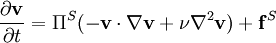 ,
,
 ,
,
 and
and  are solenoidal and irrotational projection operators satisfying
 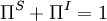 and
and
 and
and  are the nonconservative and conservative parts of the body force. This result follows from the Helmholtz Theorem . The first equation is a pressureless governing equation for the velocity, while the second equation for the pressure is a functional of the velocity and is related to the pressure Poisson equation. The explicit functional forms of the projection operator in 2D and 3D are found from the Helmholtz Theorem, showing that these are integro-differential equations, and not particularly convenient for numerical computation.
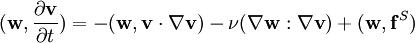 ,
,
 ,
,
 and irrotational test functions
  satisfying appropriate boundary conditions. Here, the projections are accomplished by the orthogonality of the solenoidal and irrotational function spaces. The discrete form of this is emminently suited to finite element computation of divergence-free flow.
![\nabla\phi = \left[\frac{\partial \phi}{\partial x},\,\frac{\partial \phi}{\partial y}\right]^T, \quad
\nabla\times\phi = \left[\frac{\partial \phi}{\partial y},\,-\frac{\partial \phi}{\partial x}\right]^T.](/W/images/math/8/a/5/8a58150cd07872905de0f26ea5212055.png)