A roughness-dependent model
From CFD-Wiki
(→Algebraic eddy viscosity model) |
(→References) |
||
| Line 72: | Line 72: | ||
* {{reference-paper|author=Absi, R. |year=2006|title=[http://www.jstage.jst.go.jp/article/jscejb/62/4/62_437/_article A roughness and time dependent mixing length equation]|rest=Journal of Hydraulic, Coastal and Environmental Engineering, Japan Society of Civil Engineers, (Doboku Gakkai Ronbunshuu B), Vol. 62, No. 4, pp.437-446}} | * {{reference-paper|author=Absi, R. |year=2006|title=[http://www.jstage.jst.go.jp/article/jscejb/62/4/62_437/_article A roughness and time dependent mixing length equation]|rest=Journal of Hydraulic, Coastal and Environmental Engineering, Japan Society of Civil Engineers, (Doboku Gakkai Ronbunshuu B), Vol. 62, No. 4, pp.437-446}} | ||
| + | |||
| + | * {{reference-paper|author=Nezu, I. and Nakagawa, H. |year=1993|title=Turbulence in open-channel flows|rest=A.A. Balkema, Ed. Rotterdam, The Netherlands}} | ||
| + | |||
| + | * {{reference-paper|author=Sukhodolov A., Thiele M. and Bungartz H. |year=1998|title=Turbulence structure in a river reach with sand bed|rest=Water Resour. Res., 34, pp. 1317-1334}} | ||
| + | |||
[[Category:Turbulence models]] | [[Category:Turbulence models]] | ||
{{stub}} | {{stub}} | ||
Revision as of 12:18, 21 June 2007
Contents |
Two-equation  -
- eddy viscosity model
 | (1) |
where:

One-equation eddy viscosity model
 | (2) |
Algebraic eddy viscosity model
 | (3) |
 is the mixing length.
Algebraic model for the turbulent kinetic energy
 | (4) |
 is the shear velocity and
  a model parameter.
For steady open channel flows in local equilibrium, where the energy production is balanced by the dissipation, from the modeled k-equation [Nezu and Nakagawa (1993)] obtained a similar semi-theoretical equation.
Algebraic model for the mixing length
For local equilibrium, an extension of von Kármán’s similarity hypothesis allows to write, with equation (4) [Absi (2006)]:
 | (5) |
 ,
,  is the hydrodynamic roughness.
For a smooth wall (
 ):
):
 | (6) |
the algebraic eddy viscosity model is therefore
 | (7) |
The mean velocity profile
In local equilibrium region, we are able to find the mean velocity profile from the mixing length  and the turbulent kinetic energy
  by:
by:
 | (8) |
With equations (4) and (5), we obtain:
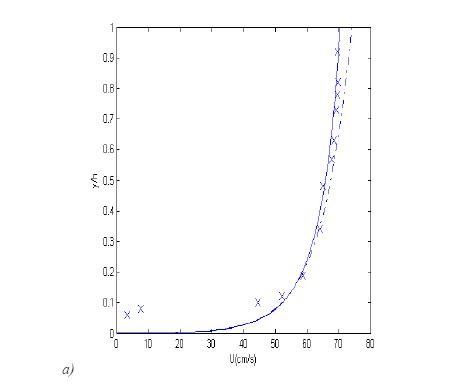
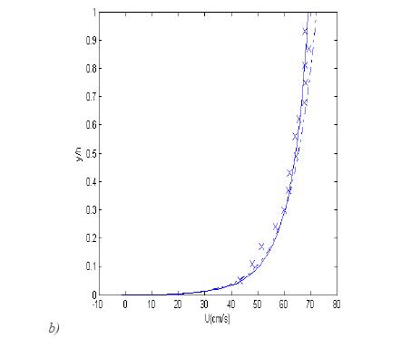
Fig. Vertical distribution of mean flow velocity.
 ;
;  ;
Dash-dotted line: logarithmic profile; solid line: obtained from equation (8); symbols: experimental data (Sukhodolov et al). a) profile 2:
  ;
;  ;
;  . b) profile 4:
  ;
;  ;
;  ; values of
  are from [Sukhodolov et al. (1998)].
References
- Absi, R. (2006), "A roughness and time dependent mixing length equation", Journal of Hydraulic, Coastal and Environmental Engineering, Japan Society of Civil Engineers, (Doboku Gakkai Ronbunshuu B), Vol. 62, No. 4, pp.437-446.
- Nezu, I. and Nakagawa, H. (1993), "Turbulence in open-channel flows", A.A. Balkema, Ed. Rotterdam, The Netherlands.
- Sukhodolov A., Thiele M. and Bungartz H. (1998), "Turbulence structure in a river reach with sand bed", Water Resour. Res., 34, pp. 1317-1334.


