RNG k-epsilon model
From CFD-Wiki
| Turbulence |
| Algebraic models |
| One equation models |
| Two equation models |
|
Contents |
Background
The RNG model was developed using Re-Normalisation Group (RNG) methods by Yakhot et al to renormalise the Navier-Stokes equations, to account for the effects of smaller scales of motion. In the standard k-epsilon model the eddy viscosity is determined from a single turbulence length scale, so the calculated turbulent diffusion is that which occurs only at the specified scale, whereas in reality all scales of motion will contribute to the turbulent diffusion. The RNG approach, which is a mathematical technique that can be used to derive a turbulence model similar to the k-epsilon, results in a modified form of the epsilon equation which attempts to account for the different scales of motion through changes to the production term.
Transport Equations
There are a number of ways to write the transport equations for k and  , a simple interpretation where bouyancy is neglected is
![\frac{\partial}{\partial t} (\rho k) + \frac{\partial}{\partial x_i} (\rho k u_i) = \frac{\partial}{\partial x_j} \left[\left(\mu+\frac{\mu_t}{\sigma_k}\right) \frac{\partial k}{\partial x_j}\right] + P_k - \rho \epsilon](/W/images/math/f/6/d/f6db20d82b6f4d9e84f9a5a1caf1c167.png)
![\frac{\partial}{\partial t} (\rho \epsilon) + \frac{\partial}{\partial x_i} (\rho \epsilon u_i) = \frac{\partial}{\partial x_j} \left[\left(\mu+\frac{\mu_t}{\sigma_{\epsilon}}\right) \frac{\partial \epsilon}{\partial x_j}\right] + C_{1 \epsilon}^*\frac{\epsilon}{k} P_k - C_{2\epsilon} \rho \frac{\epsilon^2}{k}](/W/images/math/0/0/1/0014839c22b85c053e823ee6053bea00.png)
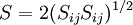
where
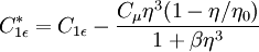
and
 and
and
With the turbulent viscosity being calculated in the same manner as with the standard k-epsilon model.
Constants
It is interesting to note that the values of all of the constants (except  ) are derived explicitly in the RNG procedure. They are given below with the commonly used values in the standard k-epsilon equation in brackets for comparison:
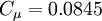 (0.09)
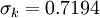 (1.0)
(1.0)
 (1.30)
 (1.44)
 (1.92)

 (derived from experiment)
Applicability and Use
Although the technique for deriving the RNG equations was quite revolutionary at the time, it's use has been more low key. Some workers claim it offers improved accuracy in rotating flows, although there are mixed results in this regard: It has shown improved results for modelling rotating cavities, but shown no improvements over the standard model for predicting vortex evolution (both these examples from individual experience). It is favoured for indoor air simulations.
References
Yakhot, V., Orszag, S.A., Thangam, S., Gatski, T.B. & Speziale, C.G. (1992), "Development of turbulence models for shear flows by a double expansion technique", Physics of Fluids A, Vol. 4, No. 7, pp1510-1520.