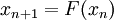
Fixed point theorem

From CFD-Wiki

(Difference between revisions)

Latest revision as of 15:25, 4 December 2006

The fixed point theorem is a useful tool for proving existence of solutions and also for convergence of iterative schemes. In fact the latter is used to prove the former. If the problem is to find the solution of

$L(u) = 0$

then we convert it to a problem of finding a fixed point

$u = F(u)$

Statement

Let $X$ be a complete metric space with distance $d(\cdot,\cdot)$ and let $F: X \to X$ be contractive, i.e., for some $0 < \alpha < 1$ ,

$d( F(x), F(y) ) \le \alpha d(x,y), \ \ \ \forall x, y \in X$

Then there exists a unique fixed point $u \in X$ such that

$u = F(u)$

Proof

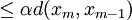
Choose any $x_o \in X$ and define the sequence $(x_n)$ by the following iterative scheme

$x_{n+1} = F(x_n)$

If we can show that the sequence $(x_n)$ has a unique limit independent of the starting value then we would have proved the existence of the fixed point. The first step is to show that $(x_n)$ is a Cauchy sequence.

$d(x_{m+1}, x_m)$	$= d(F(x_m), F(x_{m-1}))$
	$\le \alpha d( x_m, x_{m-1} )$
	$= \alpha d( F(x_{m-1}), F(x_{m-2}) )$
	$\le \alpha^2 d ( x_{m-1}, x_{m-2} )$
	$.$
	$.$
	$\le \alpha^m d(x_1, x_o)$

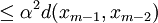
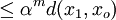
Now using the triangle inequality we get, for $n > m$

$d(x_m, x_n)$	$\le d(x_m, x_{m+1}) + d(x_{m+1}, x_{m+2}) + .... + d(x_{n-1},x_n)$
	$\le (\alpha^m + \alpha^{m+1} + .... + \alpha^{n-1} ) d(x_o, x_1)$
	$= \alpha^m \frac{ 1 - \alpha^{n-m} }{1 - \alpha} d(x_o, x_1)$
	$\le \frac{ \alpha^m }{1 - \alpha} d(x_o, x_1)$

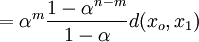
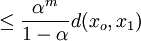
where the last inequality follows because 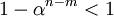$1 - \alpha^{n-m} < 1$ . Now since $\alpha^m \to 0$ as $m \to \infty$ we see that

$d(x_m, x_n) \to 0, \ \ \ \textrm{ as } \ \ \ m,n \to \infty$

which proves that $(x_n)$ is a Cauchy sequence. Since $X$ is complete, this sequence converges to a unique limit $u$ . It is now left to show that the limit is a fixed point.

$d(u, F(u)) \le d(u, x_m) + d(x_m, F(u)) \le d(u, x_m) + \alpha d(x_{m-1}, u)$

and since $u$ is the limit of the sequence we see that the right hand side goes to zero so that

$d(u, F(u)) = 0 \ \ \ \Longrightarrow \ \ \ u = F(u)$

The uniqueness of the fixed point follows easily. Let $u$ and $\bar{u}$ be two fixed points. Then

$d(u, \bar{u} ) = d(F(u), F(\bar{u})) \le \alpha d(u, \bar{u})$

and since $0 < \alpha < 1$ we conclude that

$d(u, \bar{u}) = 0 \ \ \ \Longrightarrow \ \ \ u = \bar{u}$

Application to solution of linear system of equations

We will apply the fixed point theorem to show the convergence of Jacobi iterations for the numerical solution of the linear algebraic system

$Ax = b$

under the condition that the matrix $A$ is diagonally dominant. Assuming that the diagonal elements are non-zero, define the diagonal matrix

$D = \textrm{diag}(A_{11}, A_{22}, ...., A_{NN})$

and rewriting we get

$x = D^{-1} [ b - (A-D)x]$

which is now in the form of a fixed point problem with

$F(x) = D^{-1} [ b - (A-D)x]$

For measuring the distance between two vectors let us choose the maximum norm

$d(x,y) = \max_{j} | x_j - y_j |$

We must show that $F$ is a contraction mapping in this norm. Now

$F(x) - F(y) = - D^{-1}(A-D)(x-y)$

so that the j'th component is given by

$[F(x) - F(y)]_j = \sum_{k \ne j} \frac{ A_{jk} }{ A_{jj}} (x_k - y_k)$

From this we get

$| [F(x) - F(y)]_j | \le \max_k | x_k - y_k | \sum_{k \ne j} \left| \frac{ A_{jk} }{ A_{jj}} \right|$

and

$d( F(x), F(y) ) \le d(x,y)\max_j \sum_{k \ne j} \left| \frac{ A_{jk} }{ A_{jj}} \right|$

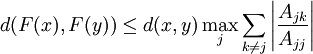
Hence the mapping is contractive if

$\sum_{k \ne j} | A_{jk} | < | A_{jj} |, \ \ \ 1 \le j \le N$

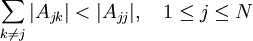
which is just the condition of diagonal dominance of matrix $A$ . Hence if the matrix is diagonally dominant then the fixed point theorem assures us that the Jacobi iterations will converge.

Application to Newton-Raphson method

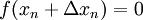
Consider the problem of finding the roots of an equation

$f(x) = 0$

If an approximation to the root $x_n$ is already available then the next approximation

$x_{n+1}= x_n + \Delta x_n$

is calculated by requiring that

$f(x_n + \Delta x_n) = 0$

Using Taylors formula and assuming that $f$ is differentiable we can approximate the left hand side,

$f(x_n) + \Delta x_n f^\prime(x_n) = 0 \ \ \ \Longrightarrow \ \ \ \Delta x_n = - \frac{f(x_n)}{ f^\prime(x_n) }$

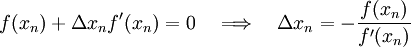
so that the new approximation is given by

$x_{n+1} = x_n - \frac{f(x_n)}{f^\prime(x_n) }$

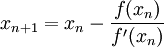
This defines the iterative scheme for Newton-Raphson method and the solution if it exists, is the fixed point of

$F(x) = x - \frac{ f(x) }{ f^\prime(x) }$

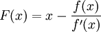
If we assume that

$(*) \quad | F^\prime(x) | \le \alpha < 1$

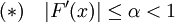
in some neighbourhood of the solution then

$F(y) - F(x) = \int^y_x F^\prime(z) d z \ \ \ \Longrightarrow \ \ \ |F(y) - F(x)| \le \alpha |y-x|$

Thus condition (*) guarantees that $F$ is contractive and the Newton iterations will converge.

Links

Fixed Point Method

@@ Line 246: / Line 246: @@
 Thus condition (*) guarantees that <math>F</math> is contractive and the
 Newton iterations will converge.
+==Links==
+[http://www.math-linux.com/spip.php?article60 Fixed Point Method]

Fixed point theorem

From CFD-Wiki

Latest revision as of 15:25, 4 December 2006

Application to solution of linear system of equations

Application to Newton-Raphson method

Links

Views

My wiki

wiki navigation

wiki search

wiki toolbox