Diffusion term
From CFD-Wiki
(→Discretisation of the Diffusion Term) |
|||
| Line 3: | Line 3: | ||
=== Description=== | === Description=== | ||
<br> | <br> | ||
| + | For a general control volume (orthogonal, non-orthogonal), the discretization of the diffusion term can be written in the following form<br> | ||
| + | <math> \int_{S}\Gamma\nabla\phi\cdot{\rm{d\vec S}} = \sum_{faces}\Gamma _f \nabla \phi _f \cdot{\rm{\vec S_f}} </math> <br> | ||
| + | where | ||
| + | *S denotes the surface area of the control volume | ||
| + | *<math>S_f</math> denotes the area of a face for the control volume | ||
| + | As usual, the subscript f refers to a given face. The figure below describes the terminology used in the framework of a general non-orthogonal control volume<br> | ||
| + | [[Image:non_orthogonal_CV_terminology.jpg]] <br> | ||
| + | '''A general non-orthogonal control volume''' <br> | ||
| + | |||
Note: The approaches those are discussed here are applicable to non-orthoganal meshes as well as orthogonal meshes. | Note: The approaches those are discussed here are applicable to non-orthoganal meshes as well as orthogonal meshes. | ||
<br> | <br> | ||
| - | A control volume in mesh is made up of set of faces enclosing it | + | A control volume in mesh is made up of set of faces enclosing it. Where '''<math>S_f</math>''' represents the magnitude of area of the face. And '''n''' represents the normal unit vector of the face under consideration. |
| - | + | ||
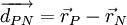
| - | + | If <math> \vec r_{P} </math> and <math> \vec r_{N} </math> are position vector of centroids of cells P and N respectively. Then, we define <br> | |
| - | + | <math> \overrightarrow{d_{PN}}= \vec r_{P} - \vec r_{N} </math> | |
| - | + | ||
| - | <math> \vec r_{ | + | |
| - | <math> | + | |
<br> | <br> | ||
| - | We wish to approaximate <math> D_f = \Gamma _f \nabla \phi _f \ | + | We wish to approaximate the diffusive flux <math> D_f = \Gamma _f \nabla \phi _f \cdot{\rm{\vec S_f}} </math> at the face. |
=== Approach 1 === | === Approach 1 === | ||
| - | + | A first approach is to use a simple expression for estimating the gradient of a scalar normal to the face. <br> | |
:<math> | :<math> | ||
| - | D_f = \Gamma _f \nabla \phi _f \ | + | D_f = \Gamma _f \nabla \phi _f \cdot \vec S_f = \Gamma _f \left[ {\left( {\phi _N - \phi _P } \right)\left| {{{\vec S_f} \over {\overrightarrow{d_{PN}}}}} \right|} \right] |
</math> <br> | </math> <br> | ||
| - | where <math> \Gamma _f </math> is suitable face | + | where <math> \Gamma _f </math> is a suitable face average. <br> |
| - | This approach is not very good when the non-orthogonality of the faces increases. | + | This approach is not very good when the non-orthogonality of the faces increases. If this is the case, it is advisable to use one of the following approaches. <br> |
=== Approach 2 === | === Approach 2 === | ||
| - | We define vector | + | We define the vector |
<math> | <math> | ||
| - | \vec \alpha {\rm{ = }}\frac{{{\rm{\vec | + | \vec \alpha {\rm{ = }}\frac{{{\rm{\vec {S_f}}}}}{{{\rm{\vec S_f}} \cdot {\overrightarrow{d_{PN}}}}} |
</math> | </math> | ||
giving us the expression: <br> | giving us the expression: <br> | ||
:<math> | :<math> | ||
| - | D_f = \Gamma _f \nabla \phi _f \ | + | D_f = \Gamma _f \nabla \phi _f \cdot{\rm{\vec S_f = }}\Gamma _{\rm{f}} \left[ {\left( {\phi _N - \phi _P } \right)\vec \alpha \cdot {\rm{\vec S_f + }}\bar \nabla \phi_f \cdot {\rm{\vec S_f - }}\left( {\bar \nabla \phi_f \cdot {\overrightarrow{d_{PN}}}} \right)\vec \alpha \cdot {\rm{\vec S_f}}} \right] |
</math> <br> | </math> <br> | ||
where <math> \bar \nabla \phi _f </math> and <math> \Gamma _f </math> are suitable face averages. <br> | where <math> \bar \nabla \phi _f </math> and <math> \Gamma _f </math> are suitable face averages. <br> | ||
Revision as of 04:36, 5 December 2005
Contents |
Discretisation of the Diffusion Term
Description
For a general control volume (orthogonal, non-orthogonal), the discretization of the diffusion term can be written in the following form
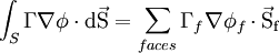
where
- S denotes the surface area of the control volume
 denotes the area of a face for the control volume
As usual, the subscript f refers to a given face. The figure below describes the terminology used in the framework of a general non-orthogonal control volume

A general non-orthogonal control volume
Note: The approaches those are discussed here are applicable to non-orthoganal meshes as well as orthogonal meshes.
A control volume in mesh is made up of set of faces enclosing it. Where represents the magnitude of area of the face. And n represents the normal unit vector of the face under consideration.
If  and
and  are position vector of centroids of cells P and N respectively. Then, we define
We wish to approaximate the diffusive flux 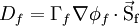 at the face.
Approach 1
A first approach is to use a simple expression for estimating the gradient of a scalar normal to the face.
![D_f = \Gamma _f \nabla \phi _f \cdot \vec S_f = \Gamma _f \left[ {\left( {\phi _N - \phi _P } \right)\left| {{{\vec S_f} \over {\overrightarrow{d_{PN}}}}} \right|} \right]](/W/images/math/2/2/f/22f7fe72fd16546ff2d65bf48adf7a35.png)
where  is a suitable face average.
This approach is not very good when the non-orthogonality of the faces increases. If this is the case, it is advisable to use one of the following approaches.
Approach 2
We define the vector

giving us the expression:
![D_f = \Gamma _f \nabla \phi _f \cdot{\rm{\vec S_f = }}\Gamma _{\rm{f}} \left[ {\left( {\phi _N - \phi _P } \right)\vec \alpha \cdot {\rm{\vec S_f + }}\bar \nabla \phi_f \cdot {\rm{\vec S_f - }}\left( {\bar \nabla \phi_f \cdot {\overrightarrow{d_{PN}}}} \right)\vec \alpha \cdot {\rm{\vec S_f}}} \right]](/W/images/math/7/c/f/7cf1e0cce420c5d8f260ea5c7f3340ff.png)
where  and are suitable face averages.
References
- Ferziger, J.H. and Peric, M. (2001), Computational Methods for Fluid Dynamics, ISBN 3540420746, 3rd Rev. Ed., Springer-Verlag, Berlin..
- Hrvoje, Jasak (1996), "Error Analysis and Estimation for the Finite Volume Method with Applications to Fluid Flows", PhD Thesis, Imperial College, University of London (download).
Return to Numerical Methods