Cebeci-Smith model
From CFD-Wiki
(Copied from B-L model, still pretty rough) |
|||
| Line 1: | Line 1: | ||
| - | == | + | == Introduction == |
| - | + | The Cebeci-Smith [[#References|[Cebeci and Smith (1967)]]] is a two-layer algebraic 0-equation model which gives the eddy viscosity, <math>\mu_t</math>, as a function of the local boundary layer velocity profile. The model is suitable for high-speed flows with thin attached boundary-layers, typically present in aerospace applications. Like the [[Baldwin-Lomax model]], this model is not suitable for cases with large separated regions and significant curvature/rotation effects (see below). Unlike the [[Baldwin-Lomax model]], this model requires the determination of of a boundary layer edge. | |
| + | == Equations == | ||
| - | ---- | + | <table width="100%"><tr><td> |
| - | < | + | :<math> |
| + | \mu_t = | ||
| + | \begin{cases} | ||
| + | {\mu_t}_{inner} & \mbox{if } y \le y_{crossover} \\ | ||
| + | {\mu_t}_{outer} & \mbox{if} y > y_{crossover} | ||
| + | \end{cases} | ||
| + | </math></td><td width="5%">(1)</td></tr></table> | ||
| + | |||
| + | where <math>y_{crossover}</math> is the smallest distance from the surface where <math>{\mu_t}_{inner}</math> is equal to <math>{\mu_t}_{outer}</math>: | ||
| + | |||
| + | <table width="100%"><tr><td> | ||
| + | :<math> | ||
| + | y_{crossover} = MIN(y) \ : \ {\mu_t}_{inner} = {\mu_t}_{outer} | ||
| + | </math></td><td width="5%">(2)</td></tr></table> | ||
| + | |||
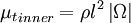
| + | The inner region is given by the Prandtl - Van Driest formula: | ||
| + | |||
| + | <table width="100%"><tr><td> | ||
| + | :<math> | ||
| + | {\mu_t}_{inner} = \rho l^2 \left| \Omega \right| | ||
| + | </math></td><td width="5%">(3)</td></tr></table> | ||
| + | |||
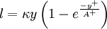
| + | where | ||
| + | |||
| + | <table width="100%"><tr><td> | ||
| + | :<math> | ||
| + | l = \kappa y \left( 1 - e^{\frac{-y^+}{A^+}} \right) | ||
| + | </math></td><td width="5%">(4)</td></tr></table> | ||
| + | |||
| + | <table width="100%"><tr><td> | ||
| + | :<math> | ||
| + | \kappa = 0.4, A^+ = 26\left[1+y\frac{dP/dx}{\rho u_\tau^2}\right]^{-1/2} | ||
| + | </math></td><td width="5%">(5)</td></tr></table> | ||
| + | |||
| + | <table width="100%"><tr><td> | ||
| + | :<math> | ||
| + | \left| \Omega \right| = \sqrt{2 \Omega_{ij} \Omega_{ij}} | ||
| + | </math></td><td width="5%">(5)</td></tr></table> | ||
| + | |||
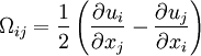
| + | <table width="100%"><tr><td> | ||
| + | :<math> | ||
| + | \Omega_{ij} = \frac{1}{2} | ||
| + | \left( | ||
| + | \frac{\partial u_i}{\partial x_j} - | ||
| + | \frac{\partial u_j}{\partial x_i} | ||
| + | \right) | ||
| + | </math></td><td width="5%">(6)</td></tr></table> | ||
| + | |||
| + | The outer region is given by: | ||
| + | |||
| + | <table width="100%"><tr><td> | ||
| + | :<math> | ||
| + | {\mu_t}_{outer} = \alpha \rho U_e \delta_v^* F_{KLEB}(y;\delta), | ||
| + | </math></td><td width="5%">(7)</td></tr></table> | ||
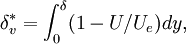
| + | |||
| + | where <math>\alpha=0.0168</math>, <math>\delta_v^*</math> is the velocity thickness given by | ||
| + | |||
| + | <table width="100%"><tr><td> | ||
| + | :<math> | ||
| + | \delta_v^* = \int_0^\delta (1-U/U_e)dy, | ||
| + | </math></td><td width="5%">(8)</td></tr></table> | ||
| + | |||
| + | and <math>F_{KLEB}</math> is the Klebanoff intermittency function given by | ||
| + | |||
| + | <table width="100%"><tr><td> | ||
| + | :<math> | ||
| + | F_{KLEB}(y;\delta) = \left[1 + 5.5 \left( \frac{y}{\delta} \right)^6 | ||
| + | \right]^{-1} | ||
| + | </math></td><td width="5%">(10)</td></tr></table> | ||
| + | |||
| + | |||
| + | == Model variants == | ||
| + | |||
| + | |||
| + | == Performance, applicability and limitations == | ||
| + | |||
| + | |||
| + | == Implementation issues == | ||
| + | |||
| + | |||
| + | == References == | ||
| + | |||
| + | *<b>Smith, A.M.O. and Cebeci, T.</b> Numerical solution of the turbulent boundary layer equations, Douglas aircraft division report DAC 33735. | ||
| + | * {{reference-book|author=Wilcox, D.C. |year=1998|title=Turbulence Modeling for CFD|rest=ISBN 1-928729-10-X, 2nd Ed., DCW Industries, Inc.}} | ||
Revision as of 18:22, 5 May 2006
Contents |
Introduction
The Cebeci-Smith [Cebeci and Smith (1967)] is a two-layer algebraic 0-equation model which gives the eddy viscosity,  , as a function of the local boundary layer velocity profile. The model is suitable for high-speed flows with thin attached boundary-layers, typically present in aerospace applications. Like the Baldwin-Lomax model, this model is not suitable for cases with large separated regions and significant curvature/rotation effects (see below). Unlike the Baldwin-Lomax model, this model requires the determination of of a boundary layer edge.
Equations
|
| (1) |
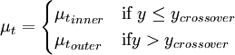
where  is the smallest distance from the surface where
  is equal to
  :
:
|
| (2) |

The inner region is given by the Prandtl - Van Driest formula:
|
| (3) |
where
|
| (4) |
|
| (5) |
![\kappa = 0.4, A^+ = 26\left[1+y\frac{dP/dx}{\rho u_\tau^2}\right]^{-1/2}](/W/images/math/d/c/1/dc17c22b20b697ea91c81fe2827b5ef7.png)
|
| (5) |
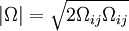
|
| (6) |
The outer region is given by:
|
| (7) |

where  ,
,  is the velocity thickness given by
|
| (8) |
and  is the Klebanoff intermittency function given by
|
| (10) |
![F_{KLEB}(y;\delta) = \left[1 + 5.5 \left( \frac{y}{\delta} \right)^6
\right]^{-1}](/W/images/math/4/3/3/4331b74159c7e4947a91a3c15e2c8282.png)
Model variants
Performance, applicability and limitations
Implementation issues
References
- Smith, A.M.O. and Cebeci, T. Numerical solution of the turbulent boundary layer equations, Douglas aircraft division report DAC 33735.
- Wilcox, D.C. (1998), Turbulence Modeling for CFD, ISBN 1-928729-10-X, 2nd Ed., DCW Industries, Inc..