Baldwin-Lomax model
From CFD-Wiki
| Line 1: | Line 1: | ||
| - | The Baldwin-Lomax model is a two-layer algebraic model which gives <math>\mu_t</math> as a function of the local boundary layer velocity profile | + | The Baldwin-Lomax model is a two-layer algebraic model which gives the eddy-viscosity <math>\mu_t</math> as a function of the local boundary layer velocity profile: |
<table width="100%"><tr><td> | <table width="100%"><tr><td> | ||
:<math> | :<math> | ||
| - | \mu_t = | + | \mu_t = |
| - | \begin{ | + | \begin{cases} |
| - | {\mu_t}_{inner} & y \ | + | {\mu_t}_{inner} & \mbox{if } y \le y_{crossover} \\ |
| - | {\mu_t}_{outer} & y > y_{crossover} | + | {\mu_t}_{outer} & \mbox{if} y > y_{crossover} |
| - | \end{ | + | \end{cases} |
| - | + | ||
</math></td><td width="5%">(1)</td></tr></table> | </math></td><td width="5%">(1)</td></tr></table> | ||
| Line 29: | Line 28: | ||
<table width="100%"><tr><td> | <table width="100%"><tr><td> | ||
:<math> | :<math> | ||
| - | + | l = k y \left( 1 - e^{\frac{-y^+}{A^+}} \right) | |
| - | l = k y \left( 1 - | + | |
</math></td><td width="5%">(4)</td></tr></table> | </math></td><td width="5%">(4)</td></tr></table> | ||
| Line 60: | Line 58: | ||
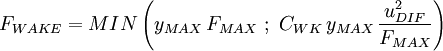
F_{WAKE} = MIN \left( y_{MAX} \, F_{MAX} \,\,;\,\, | F_{WAKE} = MIN \left( y_{MAX} \, F_{MAX} \,\,;\,\, | ||
C_{WK} \, y_{MAX} \, \frac{u^2_{DIF}}{F_{MAX}} \right) | C_{WK} \, y_{MAX} \, \frac{u^2_{DIF}}{F_{MAX}} \right) | ||
| - | </math></td><td width="5%">( | + | </math></td><td width="5%">(8)</td></tr></table> |
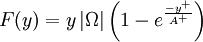
<math>y_{MAX}</math> and <math>F_{MAX}</math> are determined from the maximum of the function: | <math>y_{MAX}</math> and <math>F_{MAX}</math> are determined from the maximum of the function: | ||
| - | <table width="100%"><tr><td>:<math> | + | <table width="100%"><tr><td> |
| - | + | :<math> | |
| - | F(y) = y \left| \Omega \right| \left(1- | + | F(y) = y \left| \Omega \right| \left(1-e^{\frac{-y^+}{A^+}} \right) |
| - | </math></td><td width="5%">( | + | </math></td><td width="5%">(9)</td></tr></table> |
<math>F_{KLEB}</math> is the intermittency factor given by: | <math>F_{KLEB}</math> is the intermittency factor given by: | ||
| - | <table width="100%"><tr><td>:<math> | + | <table width="100%"><tr><td> |
| + | :<math> | ||
F_{KLEB}(y) = \left[1 + 5.5 \left( \frac{y \, C_{KLEB}}{y_{MAX}} \right)^6 | F_{KLEB}(y) = \left[1 + 5.5 \left( \frac{y \, C_{KLEB}}{y_{MAX}} \right)^6 | ||
\right]^{-1} | \right]^{-1} | ||
| - | </math></td><td width="5%">( | + | </math></td><td width="5%">(10)</td></tr></table> |
<math>u_{DIF}</math> is the difference between maximum and minimum speed in the profile. For boundary layers the minimum is always set to zero. | <math>u_{DIF}</math> is the difference between maximum and minimum speed in the profile. For boundary layers the minimum is always set to zero. | ||
| - | <table width="100%"><tr><td>:<math> | + | <table width="100%"><tr><td> |
| + | :<math> | ||
u_{DIF} = MAX(\sqrt{u_i u_i}) - MIN(\sqrt{u_i u_i}) | u_{DIF} = MAX(\sqrt{u_i u_i}) - MIN(\sqrt{u_i u_i}) | ||
| - | </math></td><td width="5%">( | + | </math></td><td width="5%">(11)</td></tr></table> |
| + | |||
| + | |||
| + | == Model constants == | ||
| + | |||
| + | The table below gives the model constants present in the formulas above. Note that <math>k</math> is a constant, and not the turbulence energy, as in other sections. It should also be pointed out that when using the Baldwin-Lomax model the turbulence energy, <math>k</math>, present in the governing equations, is set to zero. | ||
| - | + | <table cellpadding="5" cellspacing="1" border="1"> | |
| - | + | <tr> | |
| - | + | <td><math>A^+</math></td> | |
| - | + | <td><math>C_{CP}</math></td> | |
| - | <math>A^+<math> | + | <td><math>C_{KLEB}</math></td> |
| - | + | <td><math>C_{WK}</math></td> | |
| - | 26 | + | <td><math>k</math></td> |
| - | + | <td><math>K</math></td> | |
| - | + | </tr> | |
| - | + | <tr> | |
| - | + | <td>26</td> | |
| - | + | <td>1.6</td> | |
| + | <td>0.3</td> | ||
| + | <td>0.25</td> | ||
| + | <td>0.4</td> | ||
| + | <td>0.0168</td> | ||
| + | </tr> | ||
| + | </table> | ||
| - | |||
== References == | == References == | ||
| - | ''Thin Layer Approximation and Algebraic Model for Separated Turbulent Flows'' by B. S. Baldwin and H. Lomax, AIAA Paper 78-257, 1978 | + | * ''Thin Layer Approximation and Algebraic Model for Separated Turbulent Flows'' by B. S. Baldwin and H. Lomax, AIAA Paper 78-257, 1978 |
Revision as of 12:28, 8 September 2005
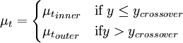
The Baldwin-Lomax model is a two-layer algebraic model which gives the eddy-viscosity  as a function of the local boundary layer velocity profile:
|
| (1) |
Where  is the smallest distance from the surface where
  is equal to
  :
:
|
| (2) |

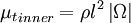
The inner region is given by the Prandtl - Van Driest formula:
|
| (3) |
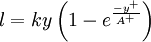
Where
|
| (4) |
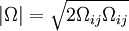
|
| (5) |
|
| (6) |
The outer region is given by:
|
| (7) |

Where
|
| (8) |
 and
and  are determined from the maximum of the function:
|
| (9) |
 is the intermittency factor given by:
|
| (10) |
![F_{KLEB}(y) = \left[1 + 5.5 \left( \frac{y \, C_{KLEB}}{y_{MAX}} \right)^6
\right]^{-1}](/W/images/math/9/b/d/9bde77641b7e232fa3e083d3e59795c4.png)
 is the difference between maximum and minimum speed in the profile. For boundary layers the minimum is always set to zero.
|
| (11) |

Model constants
The table below gives the model constants present in the formulas above. Note that  is a constant, and not the turbulence energy, as in other sections. It should also be pointed out that when using the Baldwin-Lomax model the turbulence energy, , present in the governing equations, is set to zero.
 |
 |
 |
 |
|
 |
| 26 | 1.6 | 0.3 | 0.25 | 0.4 | 0.0168 |
References
- Thin Layer Approximation and Algebraic Model for Separated Turbulent Flows by B. S. Baldwin and H. Lomax, AIAA Paper 78-257, 1978