Approximation Schemes for convective term - structured grids - Summary of Discretizations Schemes and examples

From CFD-Wiki

(Difference between revisions)

Latest revision as of 05:56, 21 April 2012

When we shall fill this page, we offer to make common identifications and definitions, because in different issues was used different notation.

Also we beg everybody to help us with original works. Please see section about what we need. If anyone have literature connected with convective schemes, please drop us a line. Of course You are welkome to participate in Wiki

We shall be very glad and grateful to hear any critical suggestion (please drop a few lines at Wiki Forum)

It is just a skeleton, but we hope that it will be developed into the good thing

1 Discretizations Schemes - Estimation of critical Peclet number
2 Discretizations Schemes - Estimation of order - Richardson extrapolation
3 Selection advice
4 Comparison of Discretizations Schemes
5 Numerical examples
- 5.1 Pure convection of a scalar step by a rotating velocity field (Smith-Hutton problem)
- 5.2 Square Lid-driven cavity flow
6 Example code for solving Smith-Hutton problem

Discretizations Schemes - Estimation of critical Peclet number

Discretizations Schemes - Estimation of order - Richardson extrapolation

William L. Oberkampf, Timothy G. Trucano (2002) Verification and validation in Computational Fluid Dynamics

Roache PJ.(1998) Verification and validation in computational science and engineering. Albuquerque, NM: Hermosa Publishers

Alvin KF, Oberkampf WL, Rutherford BM, Diegert KV.(2000) Methodology for characterizing modeling and discretization uncertainties in computational simulation. SAND2000-0515, Sandia National Laboratories, Albuquerque, NM.

We discuss a posteriori error estimation through the use of Richardson extrapolation (Roache PJ.1998). An elegant and concise discussion of this topic within a larger context of characterizing modeling uncertainties can also be found in (Alvin KF, Oberkampf WL, Rutherford BM, Diegert KV.2000). To illustrate the challenges, we focus on grid convergence extrapolation as discussed in (Alvin KF, Oberkampf WL, Rutherford BM, Diegert KV.2000). Consider for simplicity a steady-state computational problem in one spatial dimension with uniform mesh spacing $h$ : We must make several assumptions in order to perform Richardson extrapolation in a straightforward way:

Assumption 1: $\varphi$ is a smooth solution (existence of sufficient derivatives to justify the application of a Taylor expansion in the mesh spacing) of the exact PDEs.

Assumption 2: The formal convergence order $p$ of the spatial discretization method is known a priori. In addition, it is assumed that the computer code has empirically demonstrated convergence order $p$ .

Assumption 3: The mesh spacing is small enough that the leading-order error term dominates the total discretization error. This is also called the asymptotic range of the discretization (Roache PJ. 1998). One key implication of this is that convergence is monotone in the asymptotic range.

Thus, under these assumptions, expand the exact solution of the PDE of interest as

$\varphi_{exact} \left( \vec{x}\right) = \varphi_{h} \left( \vec{x}\right) + \alpha h^{p} + O \left(h^{p+1} \right)$

(1)

$\varphi_{exact} = \varphi_{h_{1}} + \alpha h^{p}_{1} + O \left(h^{p+1}_{1} \right)$

(2a)

$\varphi_{exact} = \varphi_{h_{2}} + \alpha h^{p}_{2} + O \left(h^{p+1}_{2} \right)$

(2b)

$\alpha = \left[ \frac{\varphi_{h_{1}} - \varphi_{h_{2}}}{ h^{p}_{2} - h^{p}_{1}} \right] + O \left(h^{p+1}_{1} \right) + O \left(h^{p+1}_{2} \right)$

(3)

$\varphi_{exact} = \left[ \frac{h^{p}_{2}\varphi_{h_{1}} - h^{p}_{1}\varphi_{h_{2}} }{h^{p}_{2} - h^{p}_{1}} \right] + O \left(h^{p+1}_{1} \right) + O \left(h^{p+1}_{2} \right)$

(4)

$\left\| \varphi_{exact} - \varphi_{h_{1}} \right\| \cong \left| \left[ \frac{\varphi_{h_{2}} - \varphi_{h_{1}}}{h^{p}_{2} - h^{p}_{1}} \right]h^{p}_{1} \right| + O \left(h^{p+1}_{1} \right) + O \left(h^{p+1}_{2} \right)$

(5)

$\widetilde{p} = ln \left( \frac{\varphi_{h_{3}} - \varphi_{h_{2}}}{\varphi_{h_{2}}-\varphi_{h_{1}} } \right) / ln \left( r \right)$

(6)

$r= \left(h_{3}/h_{2} \right) = \left( h_{2}/h{1} \right)$

(6)

Selection advice

Comparison of Discretizations Schemes

Numerical examples

Pure convection of a scalar step by a rotating velocity field (Smith-Hutton problem)

R.M.Smith and A.G.Hutton (1982), "The numerical treatment of advection: A performance comparison of current methods", Numerical Heat Transfer, Vol. 5, p439.

This was the test problem devised for evaluating a range of numerical models of convection at the third meeting of the International Association for Hydraulic Research Working Group on Refined Modelling of flow

Sometimes it was used scalar profile with a discontinuity at $\boldsymbol{x=-0.5}$

We shall use here smooth inlet profile

This is a simple problem with a strong discontinuity in a scalar profile and flow that is not parallel to the boundaries of the domain being tested. As such it should reveal the poor convergence of the first order schemes, which exhibit false diffusion on flow that is not parallel to the grid, whilst the sharp gradient should generate oscillations in the solutions generated using the second and third order schemes.

The steady transport equation is solved in the region $-1\leq x \leq 1$ \ , \ $0 \leq y \leq 1$ , with the streamfunction being specified as

$\psi = - \left( 1 - x^{2} \right) \left( 1 - y^{2} \right)$

(1)

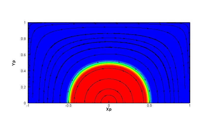
which is shown in figure below. This streamfunction gives a velocity field of

$u = 2y \left( 1 - x^{2} \right)$

(1)

$v = -2x \left( 1 - y^{2} \right)$

(1)

The scalar $\boldsymbol{\phi}$ is solved over the domain, with the value of $\boldsymbol{\phi}$ being prescribed at the inlet and on the left, right and top boundaries, whilst on the outlet the derivative of $\boldsymbol{\phi}$ normal to the boudary is set to zero. The inlet profile is given as

$\phi = 1 + \tanh \left[ \alpha \left( 2x + 1 \right) \right] \ \ \ : \ \ \ y=0 \ \ \ -1 \leq x \leq 0$

(1)

where $\boldsymbol{\alpha}$ is a parameter which defines the sharpness of the inlet profile. The outer boundaries are prescribed as

$\phi = 1 - \tanh \alpha \ \ \ : \begin{cases} x = -1 & 0 \leq y \leq 1 \\ y = 1 & - 1 \leq x \leq 1 \\ x = 1 & 0 \leq y \leq 1 \end{cases}$

(2)

Thus $\boldsymbol{\phi}$ is $\boldsymbol{0}$ on $\boldsymbol{x\pm 1 }$ and $\boldsymbol{y=1}$ , and is $\boldsymbol{2}$ at the origin. At the outlet a zero normal derivative is prescribed

$\frac{d \phi}{d y}= 0 \ \ \ \ : \ \ \ \ y=0 \ \ \ \ \ 0\leq x \leq 1$

(2)

The two parameters which define the scalar field are the Peclet number, which specifies the diffusivity of the problem, and $\boldsymbol{\alpha}$ which is a parameter that defines the sharpness of the inlet profile.

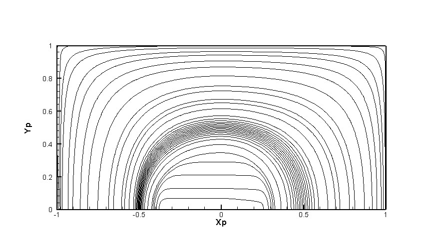
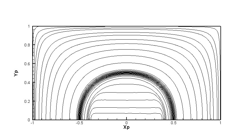
Below it's cleary seen the numerical diffusion impact, comparing the contour fields obtaining using the UDS and HLPA. A bit later we shall place here a solution gained with QUICK scheme, and it will be seen the osscilations.

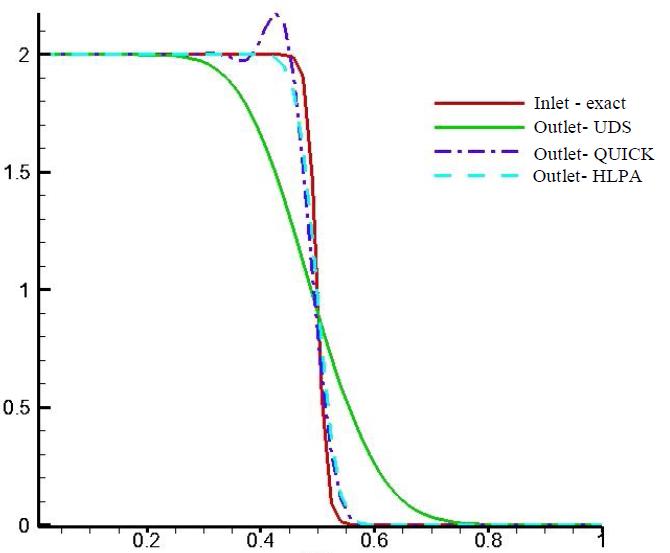
Below is the outlet profiles for solution of Smith-Hutton test. Clearly seen the diffusivity of UDS, the osscilation for QUICK scheme and it can be noticed that HLPA free of its with the same accuracy.

Square Lid-driven cavity flow

Example code for solving Smith-Hutton problem

Dear friends

It's just a scrap. Later I'll correct it, although it's a complete working code

Michail

Sample code for solving Smith-Hutton test - Fortran 90

It's results, obtained using this code (UDS and HLPA schemes)

Return to Numerical Methods

Return to Approximation Schemes for convective term - structured grids

@@ Line 11: / Line 11: @@
 == Discretizations Schemes - Estimation of critical Peclet number  ==
-== Discretizations Schemes - Estimation of order ==
+== Discretizations Schemes - Estimation of order - Richardson extrapolation ==
-== Discretizations Schemes - Estimation of error ==
+'''William L. Oberkampf, Timothy G. Trucano (2002)''' Verification and validation in Computational Fluid Dynamics
+'''Roache PJ.(1998)''' Verification and validation in computational science and engineering. Albuquerque, NM: Hermosa Publishers
+'''Alvin KF, Oberkampf WL, Rutherford BM, Diegert KV.(2000)''' Methodology for  characterizing modeling and discretization uncertainties in computational simulation. SAND2000-0515, Sandia National Laboratories, Albuquerque,
+NM.
+We discuss a posteriori error estimation through the use of Richardson extrapolation (Roache PJ.1998). An elegant and concise discussion of this topic within a larger context of characterizing modeling uncertainties can also be found in (Alvin KF, Oberkampf WL, Rutherford BM, Diegert KV.2000). To illustrate the challenges, we focus on grid convergence extrapolation as discussed in (Alvin KF, Oberkampf WL, Rutherford BM, Diegert KV.2000). Consider for simplicity a steady-state computational problem in one spatial dimension with uniform mesh spacing <math>h</math>: We must make several assumptions in order to perform Richardson extrapolation in a straightforward way:
+* Assumption 1: <math>\varphi</math> is a smooth solution (existence of sufficient derivatives to justify the application of a Taylor expansion in the mesh spacing) of the exact PDEs.
+* Assumption 2: The formal convergence order <math>p</math> of the spatial discretization method is known a priori. In addition, it is assumed that the computer code has empirically demonstrated convergence order <math>p</math>.
+* Assumption 3: The mesh spacing is small enough that the leading-order error term dominates the total discretization error. This is also called the ''asymptotic range'' of the discretization (Roache PJ. 1998). One key implication of this is that convergence is monotone in the asymptotic range.
+Thus, under these assumptions, expand the exact solution of the PDE of interest as
+<table width="100%"><tr><td>
+:<math>
+\varphi_{exact} \left( \vec{x}\right) = \varphi_{h} \left( \vec{x}\right) + \alpha h^{p} + O \left(h^{p+1} \right)
+</math>
+</td><td width="5%">(1)</td></tr></table>
+<table width="100%"><tr><td>
+:<math>
+\varphi_{exact} = \varphi_{h_{1}}  + \alpha h^{p}_{1} + O \left(h^{p+1}_{1} \right)
+</math>
+</td><td width="5%">(2a)</td></tr></table>
+<table width="100%"><tr><td>
+:<math>
+\varphi_{exact} = \varphi_{h_{2}}  + \alpha h^{p}_{2} + O \left(h^{p+1}_{2} \right)
+</math>
+</td><td width="5%">(2b)</td></tr></table>
+<table width="100%"><tr><td>
+:<math>
+\alpha = \left[ \frac{\varphi_{h_{1}} - \varphi_{h_{2}}}{ h^{p}_{2} - h^{p}_{1}} \right] + O \left(h^{p+1}_{1} \right) + O \left(h^{p+1}_{2} \right)
+</math>
+</td><td width="5%">(3)</td></tr></table>
+<table width="100%"><tr><td>
+:<math>
+\varphi_{exact} = \left[ \frac{h^{p}_{2}\varphi_{h_{1}} - h^{p}_{1}\varphi_{h_{2}} }{h^{p}_{2} - h^{p}_{1}} \right]   + O \left(h^{p+1}_{1} \right) + O \left(h^{p+1}_{2} \right)
+</math>
+</td><td width="5%">(4)</td></tr></table>
+<table width="100%"><tr><td>
+:<math>
+\left\| \varphi_{exact} - \varphi_{h_{1}} \right\| \cong \left| \left[ \frac{\varphi_{h_{2}} - \varphi_{h_{1}}}{h^{p}_{2} - h^{p}_{1}} \right]h^{p}_{1} \right| + O \left(h^{p+1}_{1} \right) + O \left(h^{p+1}_{2} \right)
+</math>
+</td><td width="5%">(5)</td></tr></table>
+<table width="100%"><tr><td>
+:<math>
+\widetilde{p} = ln \left( \frac{\varphi_{h_{3}} - \varphi_{h_{2}}}{\varphi_{h_{2}}-\varphi_{h_{1}} } \right) / ln \left( r \right)
+</math>
+</td><td width="5%">(6)</td></tr></table>
+<table width="100%"><tr><td>
+:<math>
+r= \left(h_{3}/h_{2} \right) = \left( h_{2}/h{1} \right)
+</math>
+</td><td width="5%">(6)</td></tr></table>
 == Selection advice ==
@@ Line 86: / Line 154: @@
 The two parameters which define the scalar field are the Peclet number, which specifies the diffusivity of the problem, and <math>\boldsymbol{\alpha}</math> which is a parameter that defines the sharpness of the inlet profile.
+Below it's cleary seen the numerical diffusion impact, comparing the contour fields obtaining using the UDS and HLPA. A bit later we shall place here a solution gained with QUICK scheme, and it will be seen the osscilations.
+[[Image:NM_convectionschemes_struct_grids_Smith_hutton_Countor_HLPA._probe_01.jpg]]
+[[Image:NM_convectionschemes_struct_grids_Smith_hutton_Countor_UDS_02_probe_03.jpg]]
+[[Image:NM_convectionschemes_struct_grids_Smith_hutton_Countor_HLPA_02_probe_03.jpg]]
+Below is the outlet profiles for solution of Smith-Hutton test. Clearly seen the diffusivity of UDS, the osscilation for QUICK scheme and it can be noticed that HLPA free of its with the same accuracy.
+[[Image:Outlet_profiles.JPG]]
 === Square Lid-driven cavity flow ===
@@ Line 99: / Line 178: @@
 [[Sample code for solving Smith-Hutton test - Fortran 90]]
-It's a results, obtained using this code ('''UDS''' and '''HLPA''' schemes)
+It's results, obtained using this code ('''UDS''' and '''HLPA''' schemes)
-Below it's cleary seen the numerical diffusion impact, comparing the contour fields obtaining using the UDS and HLPA. A bit later we shall place here a solution gained with QUICK scheme, and it will be seen the osscilations.
-[[Image:NM_convectionschemes_struct_grids_Smith_hutton_stream_lines_probe_01.jpg]]
-[[Image:NM_convectionschemes_struct_grids_Smith_hutton_Countor_HLPA._probe_01.jpg]]
-[[Image:NM_convectionschemes_struct_grids_Smith_hutton_Countor_HLPA_02_probe_03.jpg]]
-[[Image:NM_convectionschemes_struct_grids_Smith_hutton_Countor_UDS_02_probe_03.jpg]]
-[[Image:NM_convectionschemes_struct_grids_Smith_Hutton_Profiles_UDS_02_probe_01.jpg]]
-[[Image:NM_convectionschemes_struct_grids_Smith_Hutton_profiles_HLPA_probe_01.jpg]]

Approximation Schemes for convective term - structured grids - Summary of Discretizations Schemes and examples

From CFD-Wiki

Latest revision as of 05:56, 21 April 2012

Contents

Discretizations Schemes - Estimation of critical Peclet number

Discretizations Schemes - Estimation of order - Richardson extrapolation

Selection advice

Comparison of Discretizations Schemes

Numerical examples

Pure convection of a scalar step by a rotating velocity field (Smith-Hutton problem)

Square Lid-driven cavity flow

Example code for solving Smith-Hutton problem

Views

My wiki

wiki navigation

wiki search

wiki toolbox